Step 2: Create a Scenario and Run a DCUCOPF Optimization

Now that all pieces of the structure and topology of your model are in place, it is time to develop the scenarios and carry out the optimization. The tutorial objective is to assess the impact of the look ahead on the storage operation of the power system. In addition, you will analyze how the storage operation reduces the renewable curtailment.

Now, you will create a scenario to model a time window of a week (7 consecutive daily optimizations) with an hourly timestep resolution. In addition, you will learn how to retrieve solar and wind weather resource data from external data providers and import and include profiles. Two scenarios will be created: one with a look ahead and one without a look ahead.

1. Scenario 1 without a look ahead

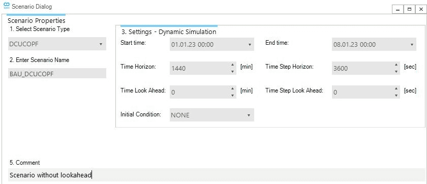
You can now develop the business-as-usual DCUCOPF scenario that you will use for understanding the storage operation without any forecast information on the following day. Thus, in this case, no look ahead is implemented. From the Scenario tab select File > New New Electric Network Scenario. Create a new DCUCOPF scenario named BAU_DCUCOPF (i.e., the business-as-usual). Set the scenario to start (StartTime) at 01/01/2023 00:00 (i.e., 00:00 a.m. on the first of January 2023). Set the scenario end time (EndTime) to 08/01/2023 00:00. The TimeHorizon is 1440 minutes, and the time step (TimeStep) is 3600 seconds, as shown in Figure 1. After filling in all the fields, click on Ok to save and create the scenario.

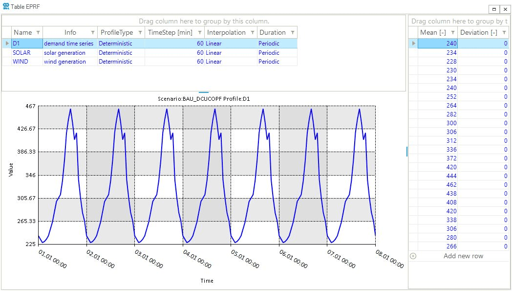
Figure 1. Scenario configuration in the dialog box.

Once the scenario is created, you need to define the profiles your external will follow during the optimization. Use deterministic profile for each external. Some profile covers one day with a hourly time step (i.e., a total of 24 steps like demand D1) while others cover seven days with an hourly time step (i.e., 168 steps like PRF_SOLAR retrieved from the data provider). The profile modeling the demand has a peak at 17:00 each day. Import the profiles using Data > Import > Profile(s) To Electric Scenario (ESCE) from the Scenario tab. Use the pre-filled profile you can find in the Excel file "Profiles_Import.xlsx" in the sub-folder .\Energy Markets\Tutorial 3 of the folder Tutorials in the directory (C:\Users\...\Documents\encoord\SAInt-v3\Projects) Figure 2 shows an example of the profiles after the import.

Figure 2. Profiles for the external objects of the third tutorial on electricity markets. Please, note that Distribution and Deviation are irrelevant for deterministic profiles.

With the following guidance, make sure to collect and generate the solar profile for the PV object. Use the how-to connect weather data, collect solar data and generate solar profile.

Finally, include the wind profile using Data > Include > Profile(s) To Electric Scenario (ESCE) from the Scenario tab. Use the .prfl file provided in the archive "Profile_Include.zip" in the sub-folder .\Energy Markets\Tutorial 3 of the folder Tutorials in the directory (C:\Users\...\Documents\encoord\SAInt-v3\Projects).

Once the profiles are loaded, open the scenario event table and add the events presented in Table 1 using either the map view or the model explorer.

Table 1. Events for the BAU_DCUCOPF scenario.
Start Time	Object Name	Parameter	Profile	Value	Unit of Measure
01/01/2023 01:00	EDEM.D1	`PSET`	D1	1	MW
01/01/2023 01:00	PV.PV	`PSET`	PRF_PV	1	MW
01/01/2023 01:00	XGEN.SOLAR	`PSET`	SOLAR	1.05	MW
01/01/2023 01:00	XGEN.WIND	`PSET`	WIND	1	MW
01/01/2023 01:00	WIND.WINDFARM	`PSET`	PRF_WIND	1	MW

Finally, you can run the scenario and check the simulation log for possible problems. If everything goes as expected, there will be no error or warning. Congratulations! Please, remember to save the project.

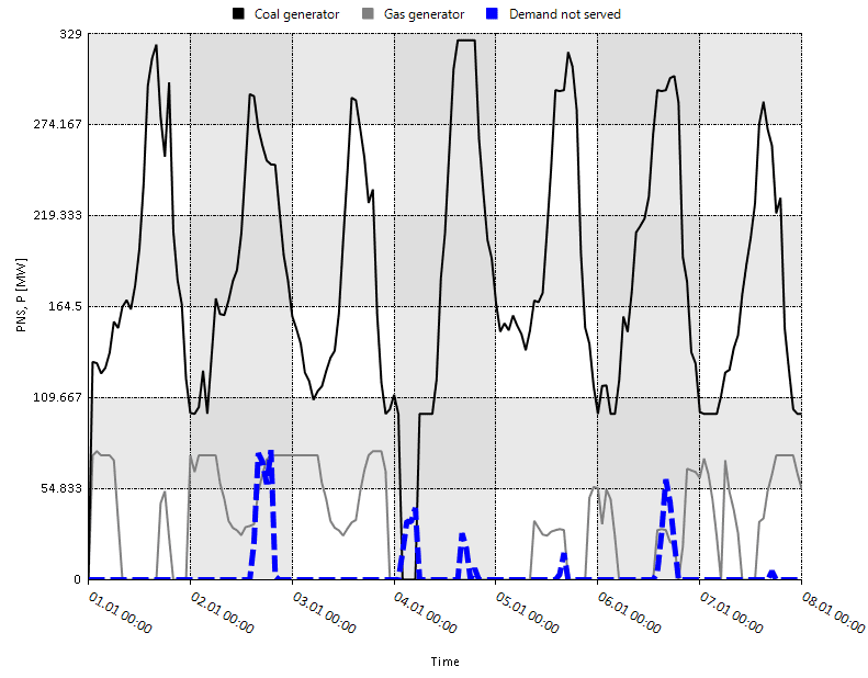
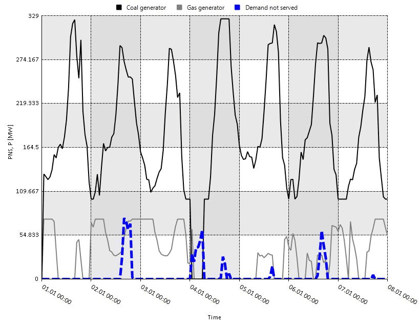
Run the new scenario and check out the demand not served and the contribution from coal and gas generators. Use the following plot command in the command window to generate Figure 3.

nplot('EDEM.D1.PNS;legend=Demand not served;blue;dash;5','FGEN.G1.P;legend=Coal generator;black','FGEN.G2.P;legend=Gas generator;gray')

Figure 3. Fuel generators' contribution to meet the demand and demand not served is shown with a dashed blue line.

1.1. A new policy is in act

Assume that the TSO operating the network is affected by a new policy limiting the total generation of fuel generators (sum of Coal and Gas) to a maximum hourly operation of 325 MW.

Before analyzing the impact of the new policy, check out how much the maximum generation from fuel generators in the previous scenario. Groups are helpful for this!

Select File > Save As Save Electric Network Scenario As to copy the scenario BAU_DCUCOPF to a new scenario called BAU_DCUCOPF_POLICY. SAInt will create a copy of the scenario and switch to it. Now you will add the policy by defining a user-defined constraint. Constraints can be defined only in network mode. Thus, close the scenario first. Add the constraint by right-clicking in the model explorer over Constraints, then menu: [Add New Constraints].

In the property editor, name the constraint "FOSSIL_FUELS_POLICY." Assign the variable P of both FGEN, right click on G1 in the model explorer and select Add New Variable Active Power Generation (P) ECNSTR.FOSSIL_FUELS_POLICY. Repeat the process for G2 to add a P variable to the newly created constraint. Rename the EVAR respectively G1 and G2.

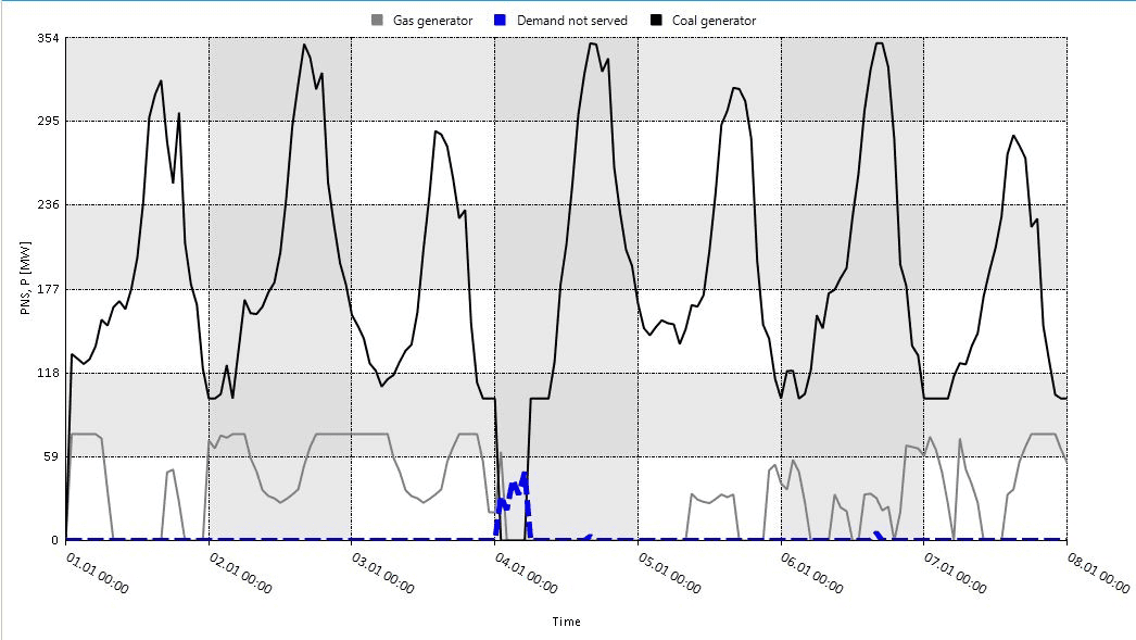
Finally, select the constraint object and set the UpBoundDef property to 325. Now you are ready to go and see the new policy’s impact on the system. Execute the scenario and repeat the same plot as before, as shown in Figure 4.

Figure 4. Fuel generators' contribution to meet the demand and demand not served is shown with a dashed blue line after the policy implementation.

You can observe a higher demand not served in the network. Evaluate if the look ahead can have an impact on the system operation.

2. Scenario 2 with look ahead

Assume the storage operator (of both X1 and X2) has invested to improve its forecasting capability. The new team now has a clearer picture of the expected demand, and the expected solar and wind generation for the following three days. This improvement will help them plan and operate the storage more efficiently.

Select File > Save As Save Electric Network Scenario As to copy the scenario BAU_DCUCOPF to a new scenario called DCUCOPF_LOOKAHEAD. Be aware that the constraint is still in place! To remove it, you can set to False the constraint’s property InService (in this case, you will keep it).

To add the look ahead, open the scenario editor Editor > ESCE Open Property Editor for Electric Scenario in pop-up Window, and change the TimeLookAhead to 72 [h], and the TimeStepLookAhead to 60 [min].

Execute the scenario and repeat the same plot as before.

The demand not served is lower on the fourth day of the simulation, as shown in Figure 5.

Figure 5. Fuel generators contribution to meet the demand, and demand not served shown as with a dash blue line after the policy implementation and look ahead of 3 days.