Analyze data

Tables in SAInt can be used to analyze results concisely, especially when you have large amounts of data. Rather than showing trends and patterns with plots, it shows the exact data values. Tables can be created both for a specific object type and combinations of object parameters to analyze and compare specific properties and results. Moreover, this data can also be analyzed from the results tab of the property editor. This tutorial focuses on analyzing some basic results using the object table and property editor.

The tables in SAInt include several functionalities to filter, search, and add conditional formatting in the object tables that can be customized using other features. A detailed explanation of all the features of object tables can be found here.

1. Object tables

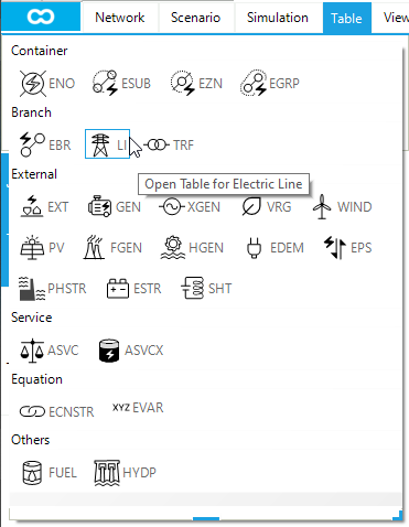
We will start by opening the electric lines (LI) table by clicking on the LI button from the table tab (Figure 1).

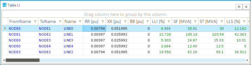
Figure 1. Access the electric lines table from the table tab.

The resulting LI table is shown in Figure 2. The table columns represent both the object’s input and output data. For example, the column with header LLI [%] represents line loading in terms of current, and PL [MW] represents active power losses. The result values in the table correspond to the display time of the map window. We can change the display time by using the time function in the command window. Enter the following expression time('01/01/2023 23:00') in the command window. Notice the change of values in the table.

Figure 2. Example of the electric line table for the last time step of the quasi-dynamic simulation.

1.1. Personalize table content

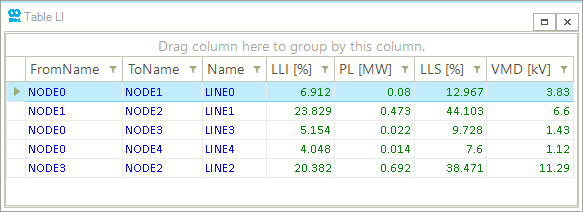
The object table’s columns are completely modifiable using the Choose Columns feature. Access the choose column dialog box by right-clicking on any of the column’s header rows and selecting Choose Columns option. In the dialog box, you will find the full list of object properties that can be shown for that specific object type. To add a column, double-click on the desired property, and for unwanted columns, you can hide them by dragging and dropping them into the dialog box. We will use the LI table to compare the following parameters: FromName, ToName, Name, LLI [%], LLS [%], VMD [kV], and PL [MW] (Figure 3).

Figure 3. Personalized electric lines table with a subset of columns.

SAInt object tables can be customized using other features. A detailed explanation of all the features of object tables can be found here.

2. Create custom tables

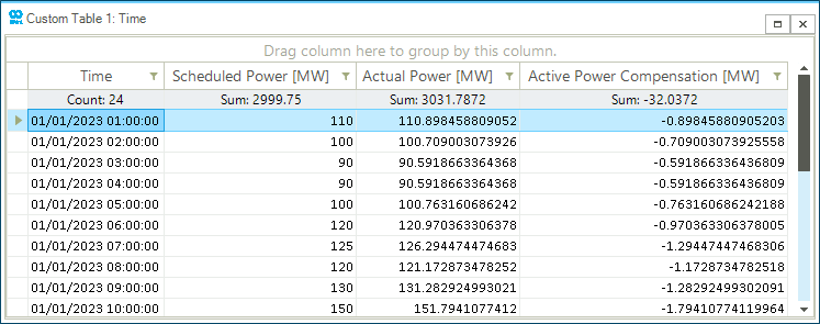
The object table can provide results for the given display time. On the other hand, the table function returns a table based on user-defined expression(s) of object parameters over a specific time window. By default, the time window is based on the chart time window, similar to the plot function. In SAInt, it is possible to analyze results from a network to an object level using the table function. For example, to analyze the active power compensation provided by the generator object NG_GEN1, you can use the following expression in the command window. Type the following expression in the command window to create the custom generator table (Figure 4).

Table expression: table('XGEN.NG_GEN1.PSET;header=Scheduled Power [MW]','XGEN.NG_GEN1.P;header=Actual Power [MW]','XGEN.NG_GEN1.PNS;header=Active Power Compensation [MW]','01/01/23 01:00','02/01/23 00:00')

Figure 4. Power flow analysis at generators level. Values are for the quasi-dynamic simulation with "Active Power Compensation Mode" set to PART.

Please refer to the tables functions section of the reference guide to learn more about the table functions' syntax, input expressions, and specifications.

2.1. Add and edit summary row

Tables can also include a summary row(s) to quickly evaluate and compare summary results between different object parameters, including values such as count, average, sum, max, and min. We can add a summary row by right-clicking on the table’s top right corner and selecting either the Toggle Show Top Summary Row or Toggle Show Bottom Summary Row option. The summary row(s) will show different summary results depending on the column or parameter data to change or view the full list of possible summary variables by right-clicking on the summary row. Notice that the top and bottom summary rows are independent of one another. Feel free to spend some time evaluating the different summary variables.

3. Property editor results tab

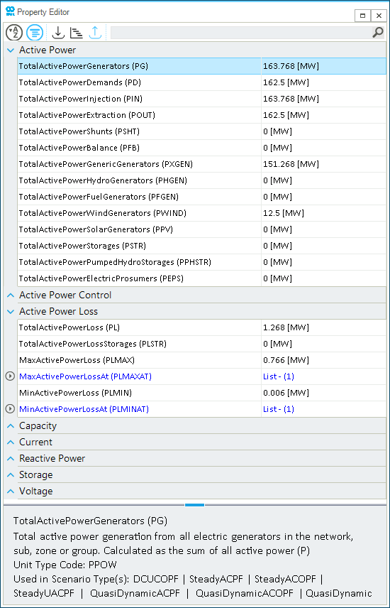
Alternatively, we can analyze the network or object results using the property editor’s results tab. We will analyze some results at the sub-network level using the property editor. Right-click the ESUB.SUB_0 object under Subs from the model explorer to access the context menu. Select Open Editor from the context menu. A sub-network property editor appears on the screen (Figure 5).

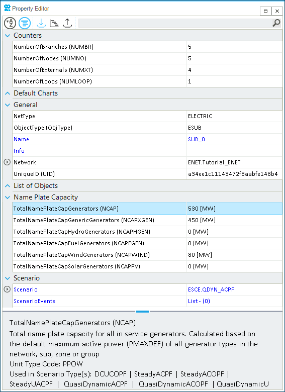
Figure 5. Electric subnetwork editor.

In the property editor, scenario input properties and results are displayed based on the display time of the map window. Access the results tab by clicking on the analyze data 06 button from the toolbar of the property editor. The expandable sections in the property editor table belong to a particular category of input properties and results. Let us collapse all the categories except the Active Power, Active Power Loss, and Current. The values of the scenario results shown in Figure 6 correspond to the last time step of the simulation, which is aligned with the display time of the map window.

Figure 6. Example of the electric subnetwork editor with results.