Step 4: Bidirectional Coupling and Loops
SAInt provides a rich array of objects to model coupling points between gas and electric systems. This intermediate-level tutorial introduces the "electric-driven gas compressor station" and the "power-to-gas" object. You can dive and learn more about these and other objects by checking the section "Hub Objects" of the reference guide for more details. In this last step of the tutorial, you will see two examples of how to strengthen bidirectional relationships in coupling objects and deploy some simple loop mechanisms. Bidirectional signals are required to improve how SAInt defines or changes an object’s "control mode." While looping allows the modeling of a fundamental mechanism of complex systems.
1. Bidirectional links
A straightforward example of a bidirectional link is provided by events of type ON or OFF. They are specially conceived to shift the control mode from one system to another.
Make sure to have your coupled system as described at the end of the third case presented in step 3 of the tutorial. You need the dynamic gas scenario H2_DYNAMIC.gsce and the electric quasi-dynamic QuasiDynamic_ACPF.esce with all the added changes.
Add to the electric scenario an event OFF to the electric demand CS1 and set the time to 02/02/2020 12:00. Add an event ON to the electric demand CS1 and set the time to 02/02/2020 14:00. These two events implement a contingency in the electric system, which is directly affecting the gas system by impacting on the way the compressor station operates.
Run the combined simulation and check the log for the messages after the time step at 14:00 on February 2. You will find a lot about how SAInt tries its best to manage the compressor station along with downstream pressure issues for some industrial customers.
Plot the behavior of EDGCS.HUB_CS1 with the following command.
nplot('HUB.HUB_CS1.POWD;left;[9,0,9];blue;title=Coupling Objects;legend=EDGCS - Driver Power', 'GCS.CS1.POWS;left;green;legend=EDGCS - Shaft Power','GCS.CS1.CTRL;right;black;legend=EDGCS - Control Mode;stepline')
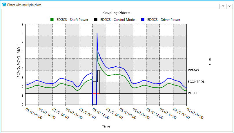
You can see in Figure 1 that the compressor station is trying to catch up as quickly as possible when electricity is again available. But, it hits the limits of its maximum compression ratio. This event creates some delays in the speed of recovery.
Save the project and close the scenarios.
2. Add a feedback loop
An example of a feedback loop can be implemented when the behavior of a coupling object on one system is modulated based on the value of a property of a different object in the other system. You will change the electric demand of the electrolyzer to maximize its send-out while complying with constraints on the final quality of the gas mixture downstream of the injection point. This approach is similar to the one presented in step 3 of the intermediate-level tutorial on gas networks, but the model reacts on the electric system based on constraints set on the gas system.
Load the dynamic gas scenario H2_DYNAMIC.gsce and the electric quasi-dynamic QuasiDynamic_ACPF.esce, and check that only the events reported in Table 1 and Table 2 are active.
| Start Time | Object Name | Parameter | Profile | Condition | Evaluation | Value | Unit of Measure |
|---|---|---|---|---|---|---|---|
01/02/2020 06:00 |
gNetwork1 |
|
NONE |
||||
01/02/2020 06:00 |
gNetwork1 |
|
NONE |
5 |
°C |
||
01/02/2020 06:00 |
PIPE4 |
|
NONE |
0 |
°C |
||
01/02/2020 06:00 |
S1 |
|
NONE |
15 |
°C |
||
01/02/2020 06:00 |
P2H2 |
|
NONE |
15 |
°C |
||
01/02/2020 06:00 |
CITY1 |
|
CITY1 |
NONE |
40 |
ksm3/h |
|
01/02/2020 06:00 |
CITY2 |
|
CITY2 |
NONE |
60 |
ksm3/h |
|
01/02/2020 06:00 |
INDUSTRY1 |
|
INDUSTRY1 |
NONE |
75 |
ksm3/h |
|
01/02/2020 06:00 |
INDUSTRY2 |
|
INDUSTRY2 |
NONE |
100 |
ksm3/h |
|
01/02/2020 06:00 |
INDUSTRY3 |
|
INDUSTRY3 |
NONE |
90 |
ksm3/h |
| Start Time | Object Name | Parameter | Profile | Condition | Evaluation | Value | Unit of Measure |
|---|---|---|---|---|---|---|---|
01/02/2020 06:00 |
WIND_FARM |
|
WIND |
NONE |
1.0 |
MW |
|
01/02/2020 06:00 |
WIND_FARM |
|
NONE |
1.0 |
MVAr |
||
01/02/2020 06:00 |
DEM1 |
|
DEM1 |
NONE |
1.0 |
MW |
|
01/02/2020 06:00 |
XGEN1 |
|
XGEN1 |
NONE |
1.0 |
MW |
|
01/02/2020 06:00 |
XGEN1 |
|
NONE |
XGEN.XGEN1.PSET |
- |
||
01/02/2020 06:00 |
XGEN1 |
|
XGEN.XGEN1==0 |
DoIFTRUE |
|||
01/02/2020 06:00 |
XGEN1 |
|
XGEN.XGEN1>0 |
DoIFTRUE |
|||
01/02/2020 06:00 |
XGEN2 |
|
XGEN2 |
NONE |
1.0 |
MW |
|
01/02/2020 06:00 |
XGEN2 |
|
NONE |
XGEN.XGEN2.PSET |
- |
Now we try to replicate a solution similar to the one obtained in the intermediate-level gas network tutorial "Contingencies and Hydrogen Blending in Transmission Systems".
Please, add the event referred in Table 3 to the electricity scenario.
| Start Time | Object Name | Parameter | Condition | Evaluation | Value | Unit of Measure |
|---|---|---|---|---|---|---|
01/02/2020 06:00 |
P2H2 |
|
NONE |
3.5446/0.65 |
MW |
|
01/02/2020 13:00 |
P2H2 |
|
GPI.PIPE4.Q*0.0516>10 |
DoIFTRUE |
54.53 |
MW |
01/02/2020 13:00 |
P2H2 |
|
GPI.PIPE4.Q*0.0516≤10 |
DoIFTRUE |
GPI.PIPE4.Q*0.0516*3.54472/0.65 |
MW |
The first event is setting the electrolyzer to produce around 1 ksm3/h of hydrogen. The value is expressed as the ratio between the equivalent of 1000 cubic meters of hydrogen at standard conditions in megawatts and the electrolyzer efficiency.
The second event is considered only when its condition is TRUE. The value of the event is set to the maximum capacity of the electrolyzer. The situation compares the "admissible amount of hydrogen" the system can blend at the maximum supply from the electrolyzer (i.e., 10 ksm3/h). The admissible amount of hydrogen must comply with a constraint stating that "the system cannot blend more than 5 % in volume of hydrogen at the node because the downstream users cannot accept higher concentration". The total inflow (QTotal) to node N6 is equal to the flow rate in pipeline 4 (QPipe) and the flow rate from the electrolyzer (QH2). The model must have 5 % x QTotal equal to QH2. But QTotal is equal to QH2 plus and QPipe. You can easily derive that QH2 is equal to 5/95 times QPipe. You have that 5/95 is approximately 0.0526. Setting a multiplier equal to 0.0516 gives you a lower blending threshold (around 4.9%).
The third event is applied when its condition is only TRUE. The value of the event is set to calculate the equivalent amount of power to produce a specific flow of hydrogen meeting the constraint of 5 % concentration in the downstream flow. The condition is the complement of the condition of the second event. The expression in the value multiplies the estimated flow of hydrogen (GPI.PIPE4.Q*0.0516) by the conversion factor to megawatt (3.54472) and divides the result for the electrolyzer efficiency (0.65).
You can see in these events how settings from one system influence the behavior of a second system, which in turn changes the first.
Once you add such new events, run the combined simulation.
|
The conversion factor is estimated by first converting the flow rate from ksm3/h to ksm3/s (i.e., divide Q by 3600). The result is multiplied by the GCV of hydrogen. This value is GCV * Q / 3600. In numbers, you have 12.761 MJ/sm3 divided by 3600 s, multiplying the flow rate Q, so it is 0.00354472 MJ/s time Q. Working with ksm3, requires multiplying this figure by 1000. |
If everything is implemented correctly, SAInt successfully completes the simulation. The log is not showing any error or warning. You can use some plots to check the systems and the constraints.
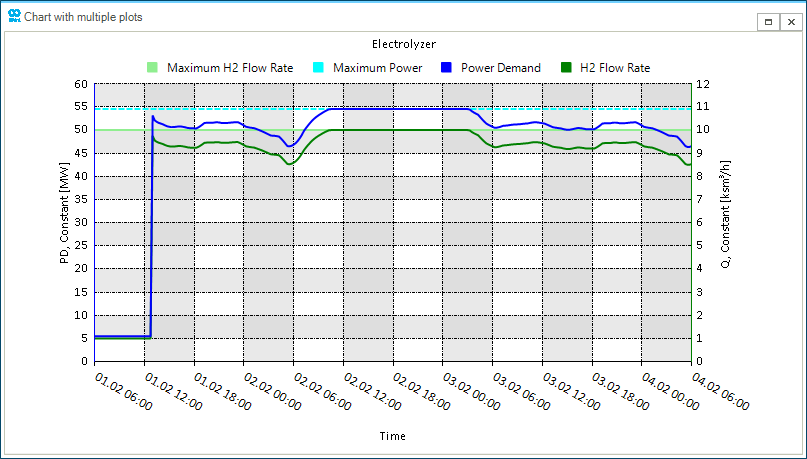
Start by plotting the electrolyzer’s power demand and the hydrogen flow rate in the gas grid. Use the following command to obtain Figure 2. You can see how the electrolyzer is used at its maximum capacity between 09:30 of 02/02/2020 and 02L30 of 03/02/2020.
nplot('HUB.HUB_P2H2.PD;[60,0,12];left;blue;legend=Power Demand;title=Electrolyzer','GSUP.P2H2.Q;[12,0,12];right;green;Legend=H2 Flow Rate','MAXFLOW[ksm3/h];lightgreen;right;legend=Maximum H2 Flow Rate','MAXFLOW2[MW];cyan;dash;left;legend=Maximum Power')
|
The |
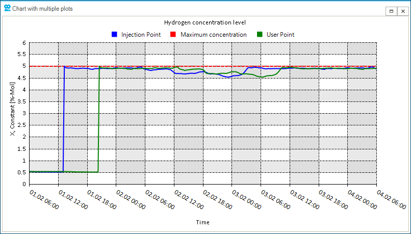
Now you can plot the molar percentage of hydrogen at the injection point and the downstream end-user INDUSTRY3. Use the following command to obtain Figure 3. You can see how the end-use downstream is not experiencing values exceeding the threshold, and there is a delay between injection and hydrogen consumption (approximately 7 hours and 15 minutes).
nplot('GNO.N7.NQ!X_H2;green;[6,0,12];title=Hydrogen concentration level;legend=User Point','GNO.N6.NQ!X_H2;blue;[6,0,12];legend=Injection Point','5[%-Mol];legend=Maximum concentration;red;dash;2')
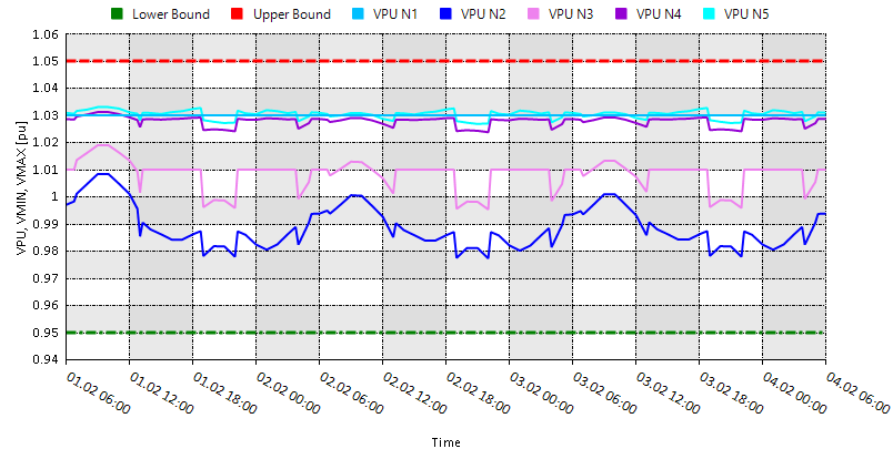
Finally, you can check the stability of the electric system by inspecting how the voltage magnitude per unit of the electric nodes changes compared to lower and upper boundary values. Use the following command to obtain Figure 4.
nplot("ENO.N1.VPU;[1.06,0.94,12];legend=VPU N1;DeepSkyBlue","ENO.N2.VPU;legend=VPU N2;Blue","ENO.N3.VPU;legend=VPU N3;Violet", "ENO.N4.VPU;legend=VPU N4;DarkViolet","ENO.N5.VPU;legend=VPU N5;Cyan","ENO.N2.VMIN;green;3;dashdot;legend=Lower Bound","ENO.N2.VMAX;red;3;dash;legend=Upper Bound")