Step 1: Visualize Data

Plots help visualize the trends and patterns in the data. The input properties and output results can be visualized with several types of plots, such as stack, scatter, and line plots. This tutorial focuses on using the pre-defined plot for the wind generator WIND_GEN3 and some custom plots for the generation mix and renewable curtailment using the plot functions in the command window of SAInt GUI.

The Default Plots for objects can be edited, saved and loaded using the Menu under Settings, Default Chart. See Default Chart (Reference-GUI-Ribbon Bar - Settings) for more information.

1. Plot time window

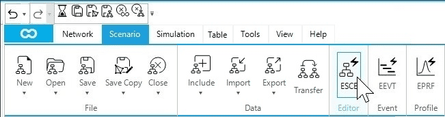
In SAInt, the plots are displayed within the pre-defined chart time window, which can be changed using the scenario editor. Before creating the plots, it is essential to adjust the chart time window based on the hours or days of interest. To change the default chart time window, open the scenario editor by clicking on ESCE from the scenario tab, as shown in Figure 1.

Figure 1. Open the scenario editor.

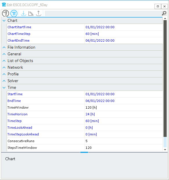
The chart time window can be adjusted by editing the ChartStartTime (start time of a plot), ChartTimeStep (time step of the plot), and ChartEndTime (end time of a plot). Your interest is to view the complete simulation results. Therefore, adjust the chart time window to be the same as the scenario time window, as shown in Figure 2.

Figure 2. Change the chart time window in the scenario editor.

2. Access the default plot

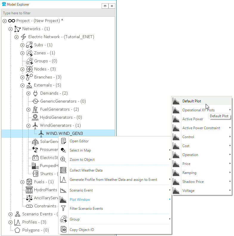
In SAInt, all the pre-defined plots for a network object are listed under the Plot Window option in the context menu. Within the pre-defined plots, the Default Plot, you can visualize a network object’s basic input properties and results. Create the default plot for the wind generator WIND_GEN3. Right-click on the WIND.WIND_GEN3 object from the model explorer (or node bar) to access the context menu. Select Plot Window Default Plot from the context menu, as shown below in Figure 3. This exact procedure can create pre-defined plots for any object type. Feel free and spend some time visualizing other objects and results.

The available options in the Plot Window will differ depending on whether a scenario file is loaded and the type of scenario.

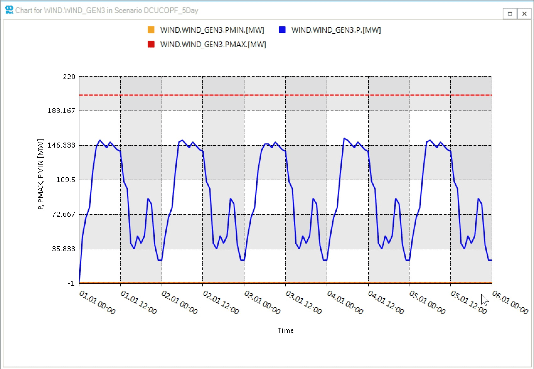
Figure 3. Plot options for WIND_GEN3 object.

The default plot of the wind generator WIND_GEN3 is created in a separate window called a chart window, as shown in Figure 4. The chart includes the nameplate capacity (PMAX), minimum active power (PMIN), and active power generation (P). The chart window has different interactive features allowing you to navigate, copy and extract the plot data. For more information on these features, please refer to the chart window section of the reference guide.

Figure 4. Default plot of WIND_GEN3 object.

3. Create customized plots

In addition to the pre-defined plots, SAInt allows users to create customized plots using multiple plot functions. You will use the results from the previous beginner tutorial to visualize the generation mix and renewable curtailment using the plot, stackplot, and nplot functions in the command window. The command window is located under the map window by default and can be opened by clicking on the Command button from the view tab.

Please refer to the plot function section of the reference guide to learn more about the plotting functions' syntax, input expressions, and specifications.

3.1. Generation mix stack plot

The Generation Mix by Production Type is a valuable plot for understanding the dispatch of the generation fleet in the day-ahead market model. In this example, you will use the network parameters PFGEN and PWIND and the stackplot function to generate this plot. The PFGEN and PWIND parameters represent the aggregated total generation per each generation type in the network. Enter the expression below in the command window to create the stackplot, as shown in Figure 5. Notice that the order of the stacking areas follows the order of expressions in the stackplot command.

`stackplot('ENET.PFGEN;indigo;legend=Fossil;title=Generation Mix by Production Type','ENET.PWIND;deepskyblue;[300,0,6];legend=Wind')`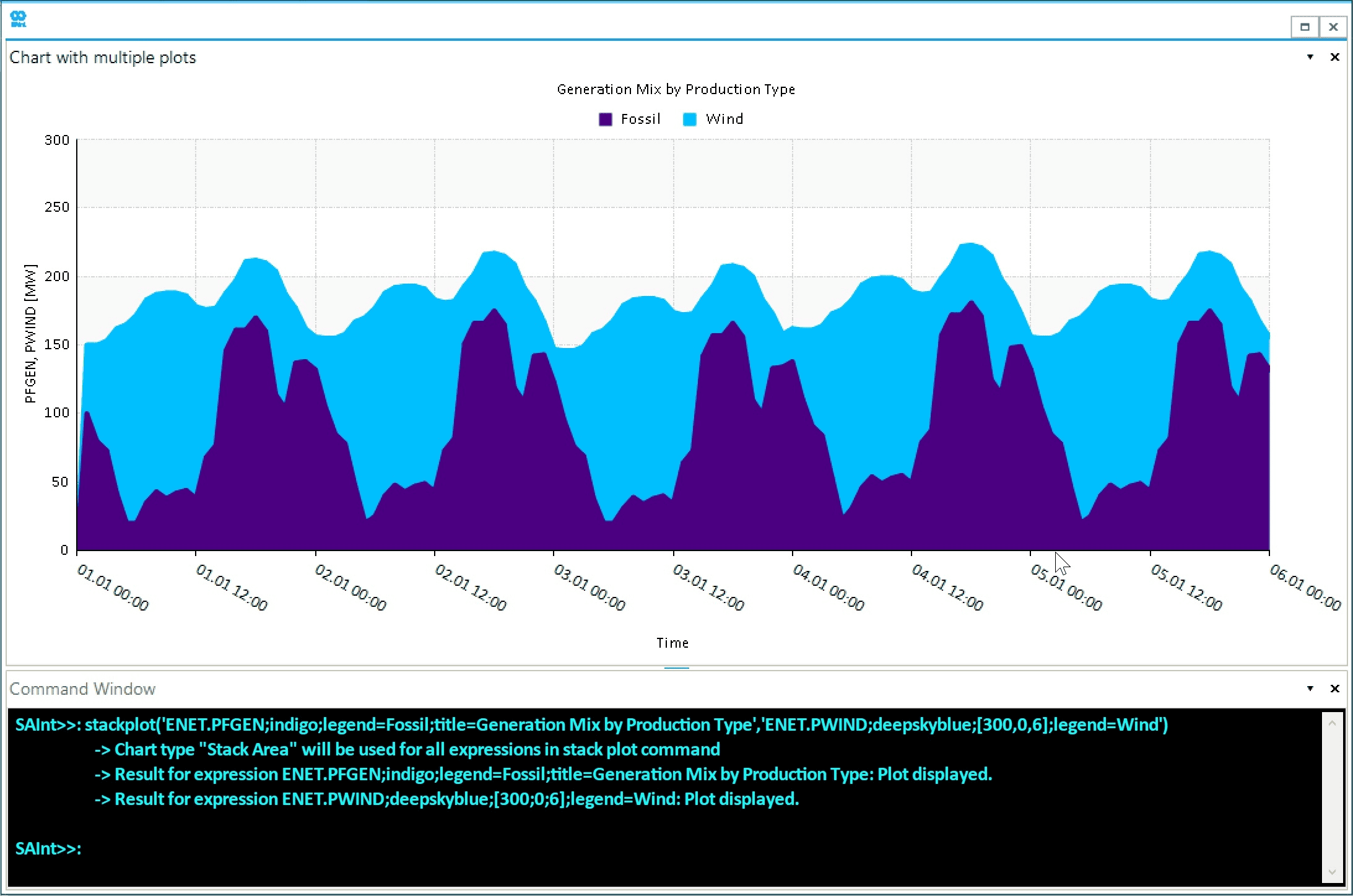

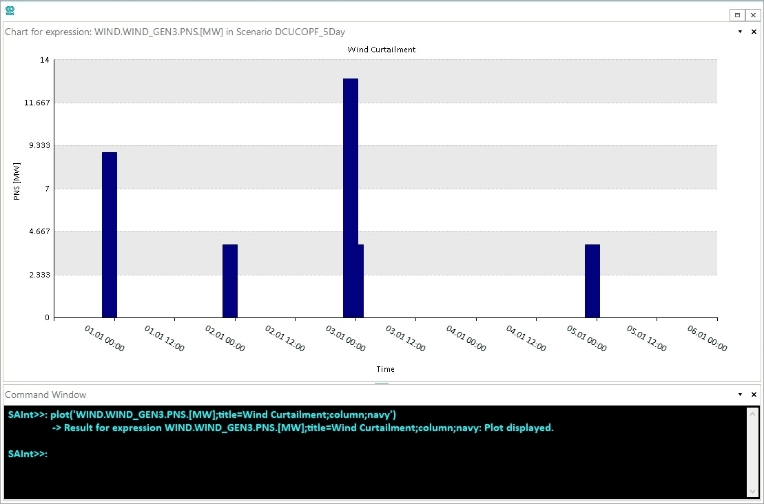
Figure 5. Generation mix by production type.

3.2. Curtailment bar plot

The Curtailment is the reduction in the output power from the maximum available capacity of a generator due to various network constraints, such as transmission congestion or excess generation during periods of low demand. The curtailment of renewable generation, such as wind and solar generators, is expected since their energy production depends on the weather conditions and does not react to the system’s demand. You will create a wind curtailment bar plot using the PNS parameter of the WIND_GEN3 generator and the plot function. The PNS is calculated by taking the difference between the setpoint power PSET and the resulting active power P. Enter the expression below in the command window to create the curtailment plot, as shown in Figure 6.

Plot expression: plot('WIND.WIND_GEN3.PNS.[MW];title=Wind Curtailment;column;navy')

Figure 6. Wind generator curtailment.

3.3. Total available generation vs. system demand

From the last plots, you can see that there are time steps with wind energy curtailment. Now, you analyze if the curtailment is due to excess generation during periods of low demand, transmission congestion, or any other reason. You will now develop a stackplot using a nplot function comparing the total available generation against the system demand. Enter the expression below in the command window to create the comparison plot, as shown in Figure 7.

Plot expression: nplot('ENET.PFGEN;indigo;stack;legend=Fossil gen.;title=Available Generation vs System Demand','ENET.PWIND;deepskyblue;stack;[300,0,6];legend=Wind gen.','WIND.WIND_GEN3.PNS;legend=Wind curt.;stack;navy','ENET.PD;legend=Demand;dash;4;R60B54G42')

Figure 7. Custom nplot.

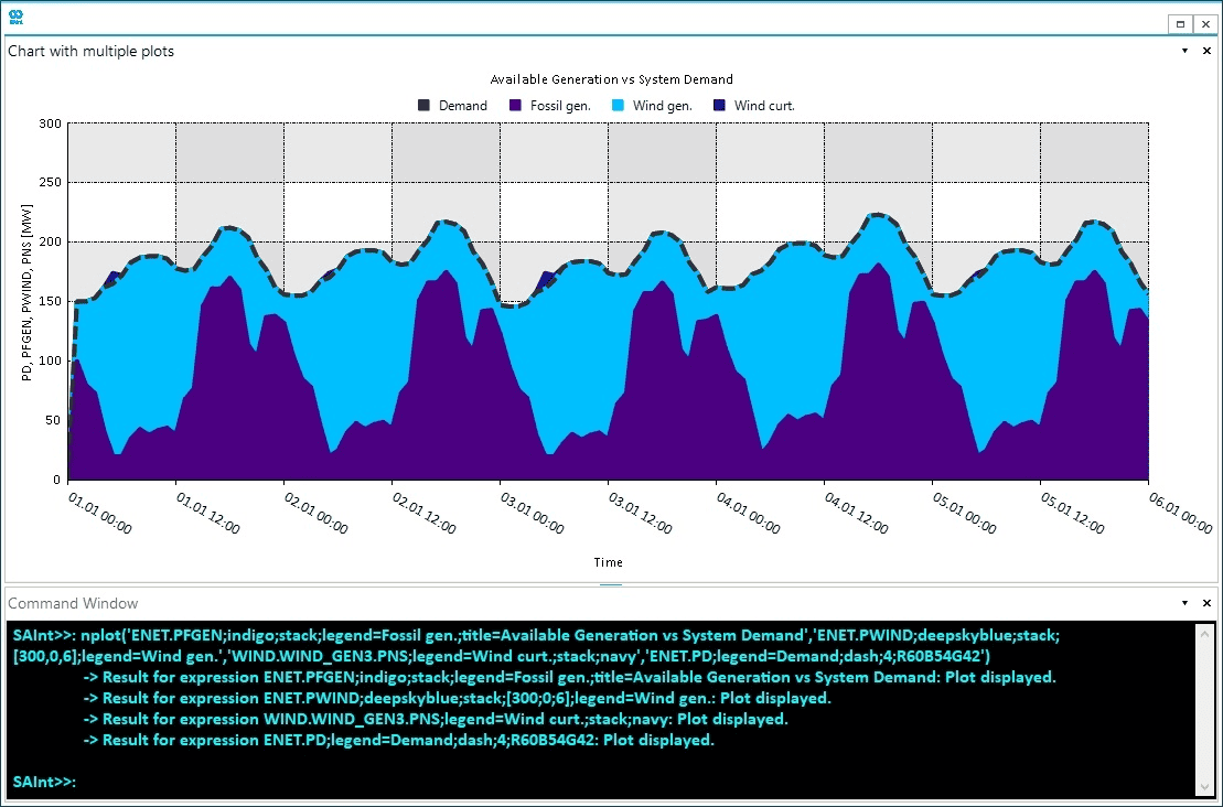
You can observe from the above plot that the wind curtailment is negligible compared to the total generation. However, wind curtailment occurs during time steps when both fuel generators operate at their full minimum capacity 20 [MW]. Therefore, the curtailment is not caused by the system demand but rather by other system constraints.

Generally, stopping and restarting fuel generators within a few hours is more expensive than paying for a few hours of curtailment because of the startup and shutdown costs. In this scenario, you have set the penalty price for wind energy curtailment to be 0 [$/MWh]. Therefore, the solver optimizes the total production cost by curtailing the wind energy for free and not paying the startup costs for the fuel generators.