Step 2: Develop a Combined Simulation Scenario

After creating a hub system, like HUBS, it is time to address the second extra step needed before running a combined simulation. You must ensure that the scenarios of all contributing networks are coherent, and aligned, and have the proper set of events.

SAInt implements a fully "combined" simulation methodology. This implies that contributing systems are not simulated in isolation and simply exchange information at coupling points. But, rather than a new single system being created, called a "hub system", a simulation can use a single set of conditions and constraints. In SAInt, you use single-energy carrier networks with their conditions, constraints, events, and scenarios. Such networks are combined in a hub system where coupling points are identified. Finally, the network scenarios are checked for coherence and alignment and merged to carry out a combined simulation.

Coherent contributing scenarios are scenarios that are of the same type. You cannot have one system described by a steady state simulation and the other by a dynamic simulation. Coherent scenarios are either only steady state scenarios or only dynamic ones.

Furthermore, contributing scenarios must be aligned. Alignment implies that all scenarios share the same start time, end time, and time step length. If dynamic, they must also have an initial state.

Finally, you learned in previous tutorials that a scenario comprises events. Such events change the behavior and state of the model’s objects and allow you to explore and assess the impact and consequences of management strategies or contingencies. But, you will see that scenarios are special in a combined simulation.

If you don’t feel conformable with some of the steps presented in this step, you can check the section scenarios and hub system of the reference guide.

1. Coherent Scenarios

Enforcing coherence is easy because SAInt will not allow combined simulation if the contributing scenarios do not meet the golden rule of "being of the same type." The user can match any steady state or dynamic scenario together. But steady state and dynamic scenarios cannot be mixed.

Suppose the button for launching a combined simulation under Execute Combined in the Simulation tab is inactive. In that case, your first check must be to have coherent scenarios loaded in your session.

So, now, it is time to load the steady state gas scenario STEADY.gsce and the electric steady state ACPF scenario Steady_ACPF.esce.

You will notice that in the Scenario tab, under the Editor and Event sections, you have active buttons for both gas and electric systems. Please, compare the two scenarios by selecting Editor GSCE and Editor ESCE. Check their properties in the property editor. For now, don’t change anything; you will do it in the next section. You can also look at the Simulation tab and see that the Execute Combined option is active.

2. Aligned Scenarios

When creating a combined scenario SAInt requires the properties under the sections Chart, Profile, Solver, and Time of the property editor of the contributing scenarios to be aligned.

When the scenarios are both steady state cases, the situation is more straightforward. Ensure the two properties, residual tolerance for linearization steps (ResidualTolerance) and maximum number of iteration steps for linearization (MaxIterationSteps), match in the Solver section. All other scenarios' properties may differ, as they do not affect the solution. In a steady state case, profiles are not used. The date and the time interval in charts are only there for visual aid. Details in the Time section are filled with values for the moment the scenario was created.

It is advisable to have the Chart section with the same values so that there is no confusion when graphs for gas and electric objects are generated. To change the values, modify the simulation’s start and end time of the simulation in the Time section, as the Chart section mirrors those values. Change the details of the electric scenario Steady_ACPF.esce to match the gas scenario STEADY.gsce. And after, create two charts by plotting PD and POWD for the compressor station.

Load now the dynamic gas scenario BAU_DYNAMIC.gsce and the quasi-dynamic electric scenario QuasiDynamic_ACPF.esce.

When the scenarios are both dynamic cases, the situation requires more work.

First, start by modifying the Solver section and matching the residual tolerance (ResidualTolerance) and the maximum number of iteration steps for linearization (MaxIterationSteps).
Second, adjust the Time section to have the same time interval and time steps to satisfy the time constraints you need for the combined simulation.
Third, focus on the Chart section and set the properties to fit your charting needs.
Fourth, address the Profile section to tune how SAInt will handle profiles. Here you can enforce a convenient rule. You can force SAInt to synchronize all profiles to the same simulation instant. Select the global profile start time (UseGlobalProfileStartTime set to True) and specify when you need your profiles to start with the global profile start time property (GlobalProfileStartTime). You can copy the values for all the options from Figure 1.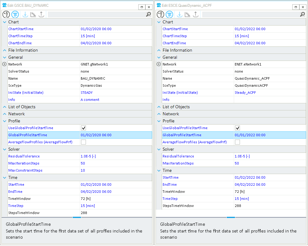

Figure 1. Values of the properties in the dynamic case for aligning the simulation scenarios.

Please now check the profiles for the gas and electric scenarios. They start at 06:00 and 00:00 on February 1, 2020.
The last fifth step is for dynamic electric scenarios, which is mandatory only when they contribute to a combined simulation. SAInt requires to have an initial state (IniState). So, select from the drop-down menu of the property IniState the value Steady_ACPF. If you forget this step, SAInt will prompt an error message that an initial state is missing when launching the combined simulation. If you don’t see the scenario in the list, you must run it and have a correct solution.

Great! You can now save your project and focus on the events of the combined simulation.

If you need more details on the properties of profiles, look at the section scenario profiles of the reference guide.

3. Events in a scenario of a combined simulation

SAInt does not require the user to create a dedicated scenario in combined simulations of coupled systems. Have a look at File New menu in the Scenario tab. You will not find the option for a "New Combined Networks Scenario"! You don’t have something similar to a *.ESCE or *.GSCE file.

Scenarios in combined simulations are special for three reasons:

First	SAInt uses and merges the events defined in the scenarios of each contributing single-energy carrier system. In this way, a "new" and "single" set of conditions and constraints is obtained and considered in the simulation. When discussing a "scenario of the combined simulation," you are considering the scenarios of the contributing systems!
Second	When members of a coupling object, the original entities from the single-energy carrier systems have some additional properties and constraints. The properties define the strength of the coupling (e.g., the efficiency factor 'Eff' for the power-to-gas conversion). The constraints set the control mode of the new object and designate which contributing system is leading the object. In the electric-driven gas compressor station, the need to compress gas defines the electricity demand, and not the availability of active power, setting how much gas it will compress in the next step. The "gas side" of the simulation controls the overall behavior of EDGCS.HUB_CS1.
Third	Events for coupling objects need to be explicitly defined in the scenario of the contributing system where the "control mode" is. Without "feedback conditions" in place or changes to the control mode, events in the other scenario are ignored. To clarify this point, open the table of the events for the steady state gas scenario STEADY.gsce and for the electric steady state ACPF scenario Steady_ACPF.esce. Now, check the events associated with EDGCS.HUB_CS1. On the gas side, an active event defines an outlet pressure set point (`POSET`) equal to 48 bar-g. On the electric side, an active event defines an active power set point (`PSET`) equal to 8 MW. Because the control mode is on the gas side, the `PSET` event is disregarded during the combined simulation, and the electric demand is defined based on the need to compress a certain amount of gas at the defined `POSET` value. You could change `PSET` to any other value, and the simulation result would not change. Similarly, the events linked to P2G.HUB_P2H2 are controlled on the electric side. The flow rate set point (`QSET`) of 1 ksm³/h is disregarded, and only the active power set point `PSET` event is enforced in the simulation. In a power-to-gas object, the demand for electricity defines the amount of gas produced, not the demand for gas setting the load on the electric system. It is recommended to set the property `Active` of an event to `False` (i.e., unselect the event) for all the events disregarded in the combined simulation for the coupling objects. This action helps improve the clarity of your events table.

Check the reference guide’s section scenarios and hub systems for details on the control mode of coupled gas-electric objects.

Temperature related events for gas entities contributing to a coupling object are not influenced by the control mode and are always enforced.