Step 1: Create the Electric Network Model

Create an electric network model using the SAInt’s extensive object library. The model has the following features:

High and low voltage grid (12.47 kV / 480 V) at 60 Hz frequency
Topology: 13 nodes, 12 branches
Externals: demands, PV generators, and a generic generator representing the upstream high-voltage grid

1. Create a new project and add your network

Start by creating a new empty project. Save it with the name acpf_intermediate in its own directory. Review the units of measurement for the project, as the tutorial uses units based on the International System. Select the euro as the currency unit.

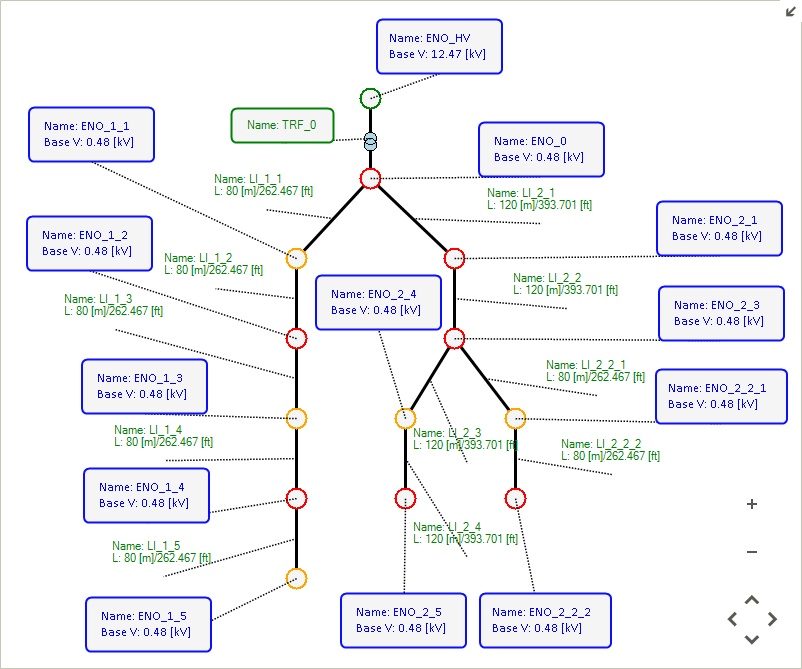
The network layout is shown in Figure 1. The network is comprised of 12 electric branches, out of which one is a transformer. Regarding the externals, there are twelve demand points, one generic generator, and five solar generators.

You can build the network yourself by referring to Figure 1 and using the details provided below, or you can make a copy of the system using the files provided in the sub-folder .\Electricity Networks\Intermediate Tutorial 1 of the folder Tutorials in the directory (C:\Users\...\Documents\encoord\SAInt-v3\Projects).

Figure 1. Diagram of the electric network used in the tutorial. The electric line lengths are not to scale.

The following tables provide the details needed to complete the network. Default values are assumed for all properties not in the tables.

Click here to view the properties of the electric network.

Table 1. Data for the electric network. The extended name and the extension of the object are reported to facilitate the editing. Extensions in bold are mandatory.
Object Name	Base apparent power	Base frequency
`Name`	`BaseS`	`BaseF`
Network_2	1 [MVA]	60 [Hz]

Click here to view the properties of the nodes.

Table 2. Data for the node objects. The extended name and the extension of the object are reported to facilitate the editing. Extensions in bold are mandatory.
Object Name	Normal voltage magnitude	Default maximum voltage magnitude	Default minimum voltage magnitude
`Name`	`BaseV`	`VMAXDEF`	`VMINDEF`
ENO_HV	12.47 [kV]	1.05 [pu]	0.95 [pu]
all other nodes	0.48 [kV]	1.05 [pu]	0.95 [pu]

Click here to view the properties of the electric lines.

Table 3. Data for the electric line objects. The extended name and the extension of the object are reported to facilitate the editing. Extensions in bold are mandatory.
Object Name	Default maximum current magnitude	Line resistance per length	Line reactance per length	Total length of the electric line	Calculate Impedances
`Name`	`IMAXDEF`	`RRL`	`XXL`	`L`	`CalcImp`
LI_1_1	500 [A]	0.2 [Ω/km]	0.08 [Ω/km]	0.08 [km]	TRUE
LI_1_2	500 [A]	0.2 [Ω/km]	0.08 [Ω/km]	0.08 [km]	TRUE
LI_1_3	500 [A]	0.2 [Ω/km]	0.08 [Ω/km]	0.08 [km]	TRUE
LI_1_4	500 [A]	0.2 [Ω/km]	0.08 [Ω/km]	0.08 [km]	TRUE
LI_1_5	500 [A]	0.2 [Ω/km]	0.08 [Ω/km]	0.08 [km]	TRUE
LI_2_1	500 [A]	0.2 [Ω/km]	0.08 [Ω/km]	0.12 [km]	TRUE
LI_2_2	500 [A]	0.2 [Ω/km]	0.08 [Ω/km]	0.12 [km]	TRUE
LI_2_2_1	105 [A]	1.5 [Ω/km]	0.3 [Ω/km]	0.08 [km]	TRUE
LI_2_2_2	105 [A]	1.5 [Ω/km]	0.3 [Ω/km]	0.08 [km]	TRUE
LI_2_3	105 [A]	1.5 [Ω/km]	0.3 [Ω/km]	0.12 [km]	TRUE
LI_2_4	105 [A]	1.5 [Ω/km]	0.3 [Ω/km]	0.12 [km]	TRUE

Click here to view the properties of the electric transformer.

Table 4. Data for the electric transformer object. The extended name and the extension of the object are reported to facilitate the editing. Extensions in bold are mandatory.
Object Name	Base voltage LV side	Base voltage HV side	Shortcircuit Voltage	Copper losses	Iron losses	Open loop losses	Calculate Impedance
`Name`	`baseLV`	`baseHV`	`VSC`	`PCU`	`PFE`	`IOL`	`CalcImp`
TRF_0	0.48 [kV]	12.47 [kV]	1.325 [%]	1 [kW]	0.95 [kW]	0.238 [%]	TRUE

3. Define properties for the externals

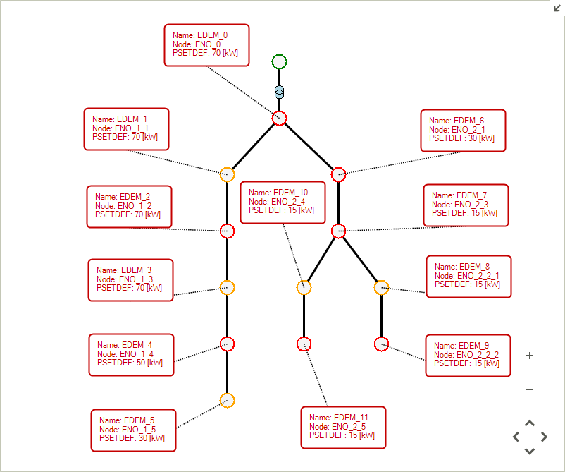
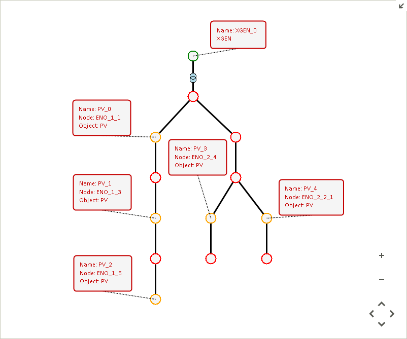
This network has three types of externals - electric demands, generic generators, and solar generators. See Figure 2 and Figure 3 for the location of these externals. Their properties are listed in the following tables.

Figure 2. Diagram showing the electric demand objects in the network.

Figure 3. Diagram showing the generator objects in the network.

Click here to view the properties of the electric demand objects.

Table 5. Data for the electric demand objects. The extended name and the extension of the object are reported to facilitate the editing. Extensions in bold are mandatory.
Object Name	Node Name	Default active power set-point	Power factor	Power factor type
`Name`	`NodeName`	`PSETDEF`	`PWF`	`PWFType`
EDEM_0	ENO_0	70 [kW]	0.957 [-]	ind
EDEM_1	ENO_1_1	70 [kW]	0.957 [-]	ind
EDEM_2	ENO_1_2	70 [kW]	0.957 [-]	ind
EDEM_3	ENO_1_3	70 [kW]	0.957 [-]	ind
EDEM_4	ENO_1_4	50 [kW]	0.957 [-]	ind
EDEM_5	ENO_1_5	30 [kW]	0.957 [-]	ind
EDEM_6	ENO_2_1	30 [kW]	0.957 [-]	ind
EDEM_7	ENO_2_3	15 [kW]	0.957 [-]	ind
EDEM_8	ENO_2_2_1	15 [kW]	0.957 [-]	ind
EDEM_9	ENO_2_2_2	15 [kW]	0.957 [-]	ind
EDEM_10	ENO_2_4	15 [kW]	0.957 [-]	ind
EDEM_11	ENO_2_5	15 [kW]	0.957 [-]	ind

Click here to view the properties of the generic generator object.

Table 6. Data for the generic generator object. The extended name and the extension of the object are reported to facilitate the editing. Extensions in bold are mandatory.
Object Name	Node Name	Default active power slack participation factor	Default voltage magnitude set point
XGEN_0	ENO_HV	1 [-]	1.04 [pu]

Click here to view the properties of the PV generator objects.

Table 7. Data for the PV generator objects. The extended name and the extension of the object are reported to facilitate the editing. Extensions in bold are mandatory.
Object Name	Node Name	Latitude	Longitude	Active power compensation factor	Tilt angle
`Name`	`NodeName`	`Lat`	`Long`	`PFSETDEF`	`Tilt`
PV_0	ENO_1_1	42.66546 [-]	-73.78246 [-]	0 [-]	40 [°]
PV_1	ENO_1_3	42.66546 [-]	-73.78246 [-]	0 [-]	40 [°]
PV_2	ENO_1_5	42.66546 [-]	-73.78246 [-]	0 [-]	40 [°]
PV_3	ENO_2_4	42.66546 [-]	-73.78246 [-]	0 [-]	40 [°]
PV_4	ENO_2_2_1	42.66546 [-]	-73.78246 [-]	0 [-]	40 [°]

Step 1: Create the Electric Network Model

1. Create a new project and add your network

2. Define properties related to network topology and structure

3. Define properties for the externals