Step 5: Run the CEM Optimization and Analyze Results

The most difficult part is done - all necessary information for solving the capacity expansion problem have been entered. All you have to do now is use SAInt-API to solve the model you have created.

1. Solve CEM model using SAInt-API

Create a Python script in the same directory as the ENET and ESCE files with the name run_cem.py. The script should contain the following code:

from ctypes import *

mydll = cdll.LoadLibrary(r"C:\Program Files\encoord\SAInt-v3\SAInt-API.dll")
mydll.evalStr('')

mydll.openENET(r"MICROGRID.ENET")
mydll.openESCE(r"CEM.esce")

mydll.showSIMLOG(True)
mydll.runESIM()

You can also use the already included script in the sub-folder .\CEM\Tutorial 1 of the folder Tutorials in the directory (C:\Users\...\Documents\encoord\SAInt-v3\Projects).

Open a terminal (Windows Command Prompt, Windows PowerShell, etc.) and change to the folder with your model. Execute the script by issuing the command python run_cem.py or py run_cem.py. SAInt will start solving the model and display informative log with the progress. When finished, you will see the message "CEM simulation completed successfully!". That’s it! You have solved your fist CEM model using SAInt.

2. Access and Analyze the Results

When the model is successfully solved, SAInt places all the output information in a folder named Output within the model directory. Since the objects that are investment candidates are PV, wind, and the storage, open AnnualOutput_PV.csv, AnnualOutput_WIND.csv, and AnnualOutput_ESTR.csv in Microsoft Excel to see the results. The screenshots below show how the results are presented in these files:

Figure 1. Results for PV.

Figure 2. Results for wind generator.

Figure 3. Results for electric storage.

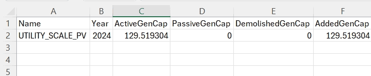
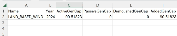
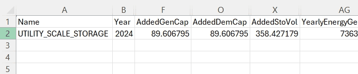
The column AddedGenCap shows the capacity (in MW) installed for the investment year. Notice that for the storage, we have more information in the AddedDemCap and AddedStoVol columns with the charging capacity (in MW) and volume (in MWh), respectively. Feel free to open the other files and see what they contain.

The Output folder also has another sub-folder called Year_00 in this example. When there are multiple investment years, we would have one sub-folder per investment year. This folder contains results related to the operation of the optimal system in the form of time-series. For example, you can analyze the amount of power imported from the upstream grid in each hour by opening the file TS_Expanded_XGEN.csv.