Step 2: Execute a DCUCOPF Scenario Using Custom Constraints and Analyze the Results

In the previous tutorial you have learned to create new custom constraint and assign new variables to these constraint. In this new series, you will perform a DCUCOPF simulation using the defined constraints and analyze the results.

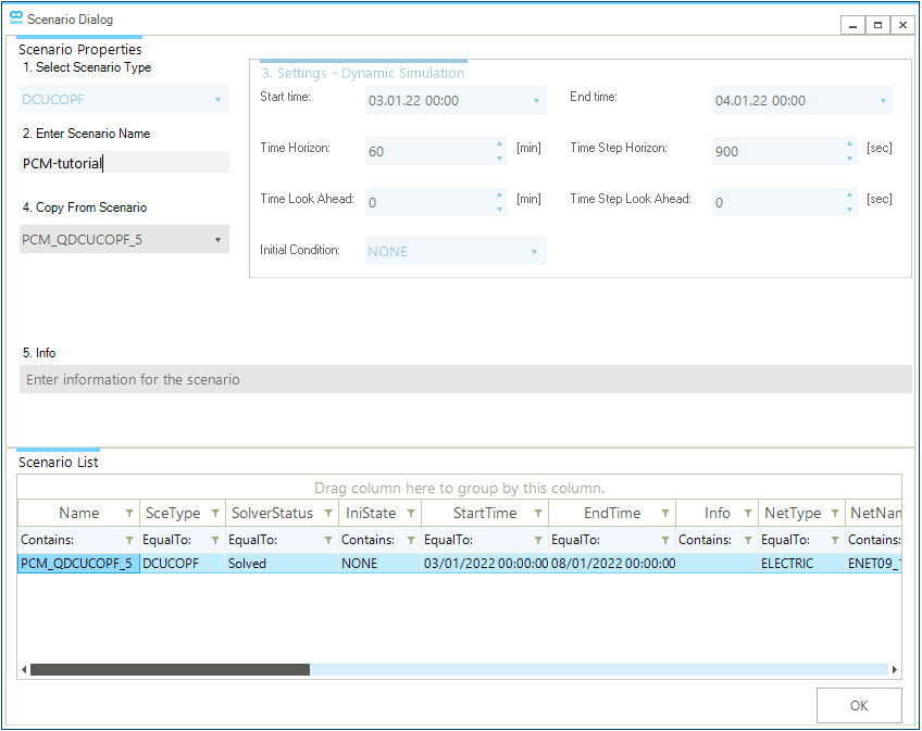
1. Create a new DCUCOPF scenario

Open SAInt and load the electric network ENET09_13 saved during the previous step, or simply continue from the end of the previous step. Click on Scenario Open Open Electric Network Scenario to access the scenario dialog. From the Scenario List, select PCM_QDCUCOPF_5 and click OK to load the scenario. Now, you will copy the scenario into a new scenario that will be used to model the implemented constraint. First click on Save As Save Electric Network As to access the Scenario Dialog, as shown in Figure 1.

Figure 1. Create a new electric scenario by saving an existing scenario.

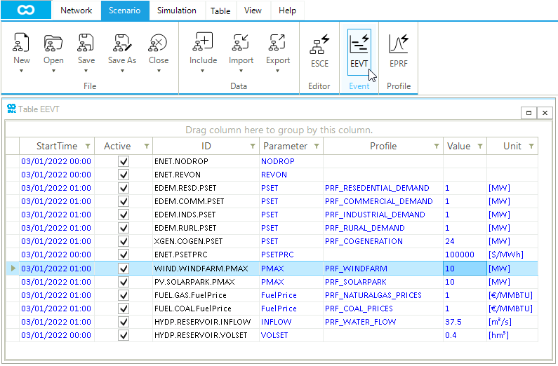
Then, enter the scenario name PCM_tutorial under the section Scenario properties, and press OK to create the new scenario, as shown in Figure 2. This process will replicate the events and profiles existing within the PCM_QDCUCOPF_5 scenario and transfer them to the newly created scenario.

Figure 2. Edit the new scenario properties in the scenario dialog.

2. Edit the scenario events

Once the new scenario is loaded, click on Scenario EEVT to open the scenario event table, as shown in Figure 3. Edit the Value property of the events WIND.WINDFARM.PMAX and PV.SOLAR.PMAX and set a value of 10 respectively, as shown in Figure 3. This procedure will increase the generation from these renewable sources, making excess energy available in the system to charge the battery.

Figure 3. Edit the events of the new scenario in the scenario event table.

3. Execute the simulation and analyze the results

Now you can execute the simulation. Go to the simulation tab and press Electric. During the scenario execution, the progress can be observed in the status bar at the bottom of the screen. Additionally, the log window will display the simulation progress during each consecutive step.

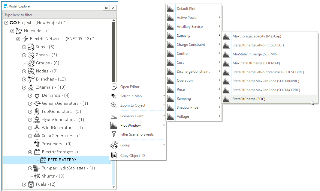
After running the simulation, you can explore the state of charge of the storage. Access the Model Explorer and right-click on the object ESTR.BATTERY. From the context menu, select Plot Window Capacity StateOfCharge (SOC), as shown in Figure 4.

Figure 4. Display the state of charge plot of the battery storage.

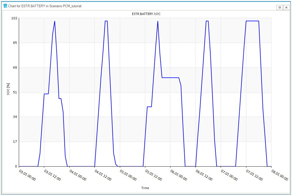
The displayed plot of the ESTR.BATTERY state of charge implemented is shown in Figure 5. The implementation of the storage state of charge incorporates a constraint on the available charging power, utilizing only the excess solar power generation.

Alternatively, you can also display the storage state of charge by copy-pasting this expression in the Command Window: plot("ESTR.BATTERY.SOC")

Figure 5. Plot of the battery storage’s state of charge.

4. Save the network

To save your work, you will need to save the new scenario file. Go to the network tab and select Save Save Electric Network Scenario. This will update the scenario file with the changes on the event values. Notice that the log window will inform you once the scenario has been saved.

Having defined constraints on the charging state of the storage and plotted its state of charge, the subsequent step involves comparing your results with the storage state of charge when no constraints are applied.