Step 3: Create and Analyze a Quasi-dynamic AC Power Flow Scenario

Open the quasi-dynamic ACPF scenario Scenario_2.esce. Remember to use the File>Open  Open Electric Network Scenario from the Scenario tab. Verify that the scenario has the StartTime set to 00:00 on 6 October 2022 and EndTime set to 23:00 on the same day. These time stamps can be found easily on the status bar at the bottom. You will use a timestep of one hour for this tutorial.

If you are building the scenario from scratch, you can add the profiles to the model using a copy of the file "electric-profiles.prfl" from the sub-folder .\Electricity Networks\Intermediate Tutorial 1 of the folder Tutorials in the directory (C:\Users\...\Documents\encoord\SAInt-v3\Projects). Select Data>Include>Profile(s)  To Electric Scenario (ESCE) from the Scenario tab and specify the location of the file. A message will confirm that the profiles have been included in the scenario. There is one profile for the electric demands and one for the PV generators. You can view the shape of the profiles by going to the profile table from the Scenario tab. Notice that the profiles are normalized to the peak value. This procedure allows you to control the value used in the simulation by using scaling factors in the event definition.

Similarly, you can add the events using a copy of the Excel file "quasi-dynamic-acpf-events.xlsx" from the sub-folder .\Electricity Networks\Intermediate Tutorial 1\Import of the folder Tutorials in the directory (C:\Users\...\Documents\encoord\SAInt-v3\Projects). Select Data>Import>Event(s)  To Electric Scenario (ESCE) from the Scenario tab and specify the location of the file. A message will inform that the events have been correctly imported to the scenario.

Open the events table for the scenario and verify the following:

Run the simulation from the Simulation tab by selecting the option Execute  Electric. SAInt will display a pop-up window on successfully completing the simulation. Make sure to have a look at the contents of the log window!

You can now take a close look at the results. First, examine if there are any voltage magnitude violations at any of the nodes. Go to the Command Window and enter the following command:

table('ENO.%.VPU')

A table opens with the voltage magnitudes of all nodes in the network. You can manually verify if the voltages are within limits. However, it would be easier if you could plot the voltage magnitudes. Plotting would also allow you to look for correlations between load, PV generation, and voltage magnitudes. You can achieve this with the following command:

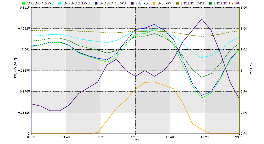
nplot('ENET.PD;left;indigo','ENET.PPV;left;orange','ENO.ENO_0.VPU;[1.06,0.94,6];right;dash;olive','ENO.ENO_1_2.VPU;right;dash;green','ENO.ENO_1_5.VPU;right;dash;lime','ENO.ENO_2_3.VPU;right;dash;cyan','ENO.ENO_2_5.VPU;right;dash;blue','06/10/2022 01:00','06/10/2022 23:00')

You can see in Figure 1 how some nodes' voltage magnitudes change with the demand. The voltage magnitudes are lower during the timesteps corresponding to peak demand and low PV generation. Despite being lower, the voltage magnitudes are within the limits of +/- 5 p.u. throughout the day.

Now take a look at the line loading using another plot. Enter the following command in the Command Window:

nplot('LI.LI_1_1.LLI;blue','LI.LI_1_5.LLI;indigo','LI.LI_2_1.LLI;cyan','LI.LI_2_4.LLI;green','06/10/2022 01:00','06/10/2022 23:00')

The plot looks like Figure 2

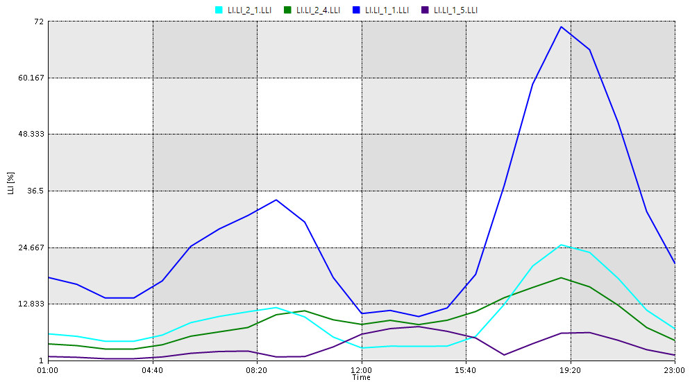
The plot makes verifying the absence of line-loading violations for the entire simulation duration easy. Feel free to use the syntax for the plots and tables to perform further analysis.

Save your project and close the opened scenarios.