Step 3: Evaluate Data
This tutorial focuses on the IronPython scripting in the script editor of SAInt GUI. It explains the procedure for developing scripts using SAInt built-in functions to evaluate input properties and results. The IronPython scripting language can be used in SAInt GUI to automatize data analysis and processing tasks. Benefits of using IronPython’s notable features include:
-
Easy to develop user-defined functions.
-
High-level programming language and easy-to-read syntax.
-
Access to all network objects and properties.
-
Usage of built-in SAInt commands (e.g., plot, table, eval, etc.).
-
Usage of third-party modules.
1. IronPython script editor
SAInt GUI has an integrated script editor which can be used to write and execute scripts.
After execution, the results are displayed in the command window, the plots and tables are created and the variables are saved in the workspace of SAInt GUI.
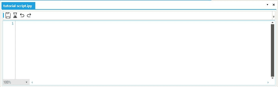
To create a new IronPython script, click on from the view tab.
A new script editor appears as a tabbed document, as shown in Figure 1.
Click on  to save the script to a user-defined location.
To execute the script, click on
to save the script to a user-defined location.
To execute the script, click on  .
.
|
An existing IronPython script can also be loaded into SAInt GUI by clicking from the view tab. The IronPython script will be saved when executed, even iff the user does not provide a custom name or location to save the file. |
2. SAInt built-in functions
SAInt has various built-in functions to be used in the script editor and command window. In the visualize data and analyze data tutorials, you learned how to use the plot and table functions in the command window. In this tutorial, you will use some of the other built-in functions in the script editor to evaluate different kinds of results. The evaluation functions (e.g., esum, emax, emean, ecount, etc.) are used to evaluate and aggregate properties and results to understand the behavior of an object within a given time step or scenario time window.
|
Please refer to the evaluation functions section of the reference guide to learn more about the evaluation functions' syntax, input, and return expressions. |
2.1. Sum of values - esum function
Evaluate the total active power generation, total production cost, and the total fuel cost of the network using the esum function.
Type the following commands in the script editor and execute them:
esum('ENET.PG.[MW].(%)')-
Returns the total active power generation of the network: 21983 [MWh].
esum('ENET.TOTCOSTRATE.[$/h].(%)')-
Returns the total production cost of the network: 602874.5 [$].
esum('ENET.CO2RATE.[t/h].(%)')-
Returns the total emission of the network: 4450.392375 [tonCO2].
|
The "e" at the beginning of the function |
2.2. Maximum value - emax function
The emax function can be used to evaluate the maximum value of an object parameter.
You use the function to determine the peak power demand of the network and the maximum shadow price at the electric node NODE1.
Type the following commands in the script editor and execute them:
emax('ENET.PDSET.[MW].(%)')-
Returns the peak power demand of the network: 223 [MW].
emax('ENO.NODE1.PSHDW.[$/MWh].(%)')-
Returns the maximum shadow price at NODE1: 54.5 [$/MWh].
2.3. Table with mean values - meantable function
In addition to the basic table function you used in the analyze data tutorial, SAInt has other table functions to tabulate results and input properties.
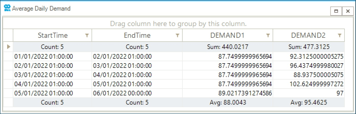
You will use the meantable function to evaluate the average power demand of both demand objects over a 24[h] period.
Use the following expression in the command window or script editor and execute.
meantable('EDEM.DEMAND2.PSET.[MW]','24[h]','01/01/22 01:00','06/01/22 00:00')-
As shown in Figure 2 the script returns a table with the daily average power demand values. Notice the start time of the function is one hour ahead of the scenario start time, which aligns with the start time of the object’s
PSETscenario event.
2.4. Graphical functions with tables - gmax and gmaxat functions
SAInt built-in graphical functions return graphical data to be used with the plot and table functions to plot and tabulate aggregated results and input properties.
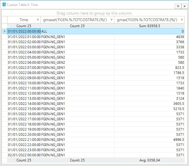
Use the gmaxat and gmax graphical functions with the table function to check which fuel generator has the maximum total cost rate at each time step during the first day of the simulation.
Type the following command in the script editor and execute:
table(gmaxat('FGEN.%.TOTCOSTRATE.(%)'),gmax('FGEN.%.TOTCOSTRATE.(%)'),'01/01/2022 00:00','02/01/2022 00:00')-
As observed in Figure 3 the table function returns the
ObjectIDof the particular fuel generator that has the maximum total cost rate and the value of the maximum total cost rate at every time-step of the simulation.