Step 2: Analyze Data
Tables in SAInt can be used to analyze results concisely, especially with large amounts of data. Rather than showing trends and patterns with plots, it shows the exact data values. Tables can be created both for a specific object type and combinations of object parameters to analyze and compare particular properties and results. Moreover, this data can also be accessed from the results tab of the property editor. This tutorial covers some fundamental results using the object table and property editor.
|
The tables in SAInt include several functionalities to filter, search, and add conditional formatting object tables that can be customized using other features. A detailed explanation of all the features of object tables can be found here. |
1. Object tables
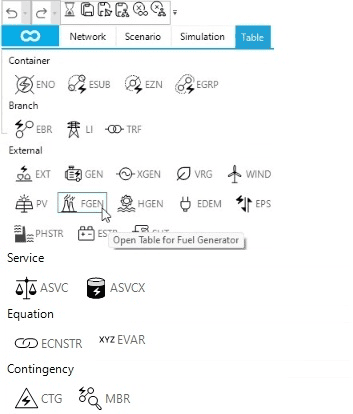
You will start by opening the fuel generator (FGEN) table by clicking on the FGEN button from the table tab, as shown in Figure 1.
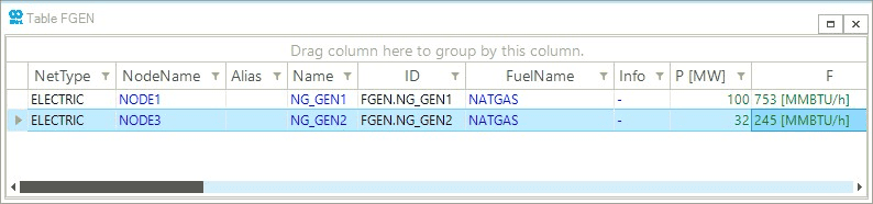
The resulting FGEN table is shown in Figure 2.
The table columns represent both the object’s input and output data.
For example, the column with header F represents fuel consumption, and P [MW] represents active power generation.
The table’s result values correspond to the map window’s display time.
You can change the display time using the time function in the command window.
Enter the following expression time('03/01/2022 14:00') in the command window.
Notice the change of values in the table.
1.1. Personalize table content
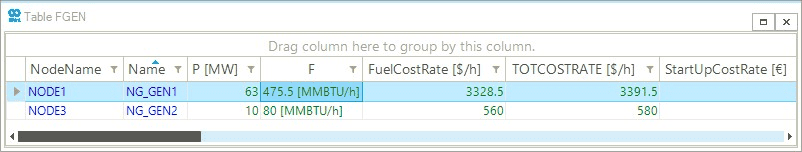
The object table’s columns are adjustable using the Choose Columns feature. Access the choose column dialog box by right-clicking on any of the column’s header rows and selecting Choose Columns option. In the dialog box, you will find the complete list of object properties that can be shown for that specific object type. To add a column, double-click on the desired property, and for unwanted columns, you can hide them by dragging and dropping them into the dialog box. Use the FGEN table to compare the following parameters:
-
NodeName -
Name -
P [MW] -
F -
FuelCostRate [$/h] -
TOTCOSTRATE [$/h] -
StartUpCostRate [$]as shown in Figure 3.
|
SAInt object tables can be customized using other features.
A detailed explanation of all the features of object tables can be found here.
The Units for |
2. Create custom tables
The object table can provide results for the given display time.
On the other hand, the table function returns a user-defined expression(s) of object parameters over a specific time window.
By default, the time window is based on the chart time window, similar to the plot function.
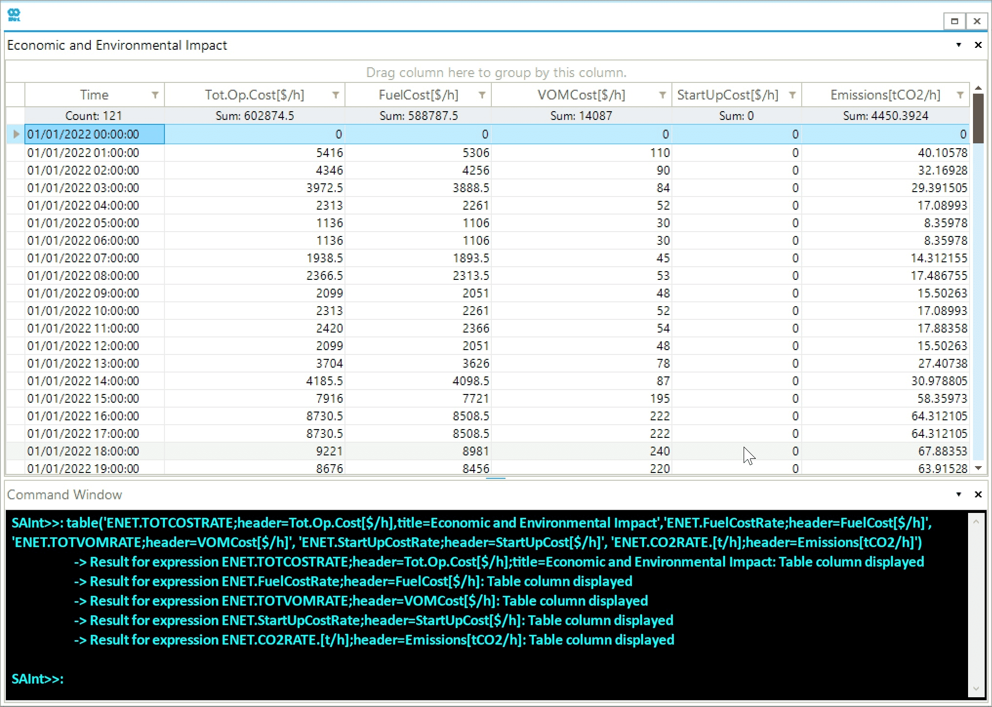
You can use the table function to evaluate the economic and environmental impact of operating the system.
In SAInt, it is possible to analyze cost and carbon emissions from a global level to specific objects.
In the following example, you will only create a table to study the evolution of the global network results.
Use the following expression in the command window to create the custom network table, as shown in Figure 4.
- Table expression
-
table('ENET.TOTCOSTRATE;header=Tot.Op.Cost[$/h],title=Economic and Environmental Impact','ENET.FuelCostRate;header=FuelCost[$/h]', 'ENET.TOTVOMRATE;header=VOMCost[$/h]', 'ENET.StartUpCostRate;header=StartUpCost[$/h]', 'ENET.CO2RATE.[t/h];header=Emissions[tCO2/h]')
|
Please refer to the tables functions section of the reference guide to learn more about the table functions' syntax, input expressions, and specifications. |
2.1. Add and edit summary row
Tables can also include a summary row(s) to quickly evaluate and compare summary results between different object parameters, including values such as count, average, sum, max, and min. You can add a summary row by right-clicking on the table’s top right corner and selecting either the Toggle Show Top Summary Row or Toggle Show Bottom Summary Row option. The summary row(s) will show different summary results depending on the column or parameter data to change or view the complete list of possible summary variables by right-clicking on the summary row. Notice that the top and bottom summary rows are independent of one another. Feel free to spend some time evaluating the different summary variables.
3. Property editor results tab
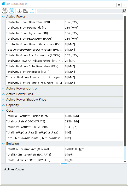
Alternatively, you can analyze the network or object results using the property editor’s results tab. You will analyze some results at the sub-network level using the property editor. Right-click the ESUB.SUB_0 object under Subs from the model explorer to access the context menu. Select Open Editor from the context menu. A sub-network property editor appears on the screen, as shown in Figure 5.
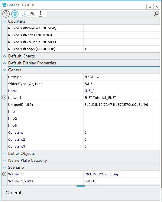
In the property editor, scenario input properties and results are displayed based on the display time of the map window.
Access the results tab by clicking on the  button from the toolbar of the property editor.
The expandable sections in the property editor table belong to a particular category of input properties and results.
Collapse all the categories except:
button from the toolbar of the property editor.
The expandable sections in the property editor table belong to a particular category of input properties and results.
Collapse all the categories except:
-
Active Power -
Cost -
Emission
The values of the scenario results shown in Figure 6 correspond to the last time step of the simulation, which is aligned with the display time of the map window.