Ribbon Bar
The ribbon bar is the main starting point to carry out many actions and tasks in SAInt. The ribbon bar is organized around three components: the "quick access" bar at the left of the title bar of the GUI, the "application menu" which can be opened from the button located in the left corner below the title bar of the GUI, and the "ribbon tabs" stretching along the main section of the window (Figure 1). From the different parts of the ribbon bar, the user can quickly execute simulations and save results and scenarios, customize all settings, or access all main panels and menu items.
1. Quick access bar
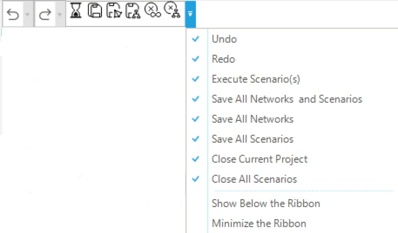
The quick access bar is shown in Figure 2. It contains the buttons of frequently used GUI functions. By default, the quick access bar is located in the top left corner of the GUI. It can be customized by selecting and deselecting the different functions from the context menu. Table 1 describes the quick access bar functions.
| Icon | Options | Description |
|---|---|---|
|
Undo |
The bent arrow undoes the last change to a property of an object. The downward arrow lists the recent changes. Only properties of objects can be modified. |
|
Redo |
The bent arrow redoes the last change to a property of an object. The downward arrow lists the recent changes. Only properties of objects can be modified. |
|
Execute Scenario(s) |
Shortcut to execute the loaded scenarios. |
|
Save All Open Network(s) and scenario(s) |
Shortcut to save both active networks and scenarios. |
|
Save All Open Network(s) |
Shortcut to save all loaded networks. |
|
Save All Open Scenario(s) |
Shortcut to save all scenarios active in the model. |
|
Close Current Project |
Shortcut to close the current project. |
|
Close All Open Scenario(s) |
Shortcut to close all scenarios active in the model. |
|
Customization |
Shows the list of available options. Checked options are displayed in the quick access bar. The position of the quick bar can be customized by selecting above or below the ribbon bar. |


|
Multiple changes can be modified at once from Undo and Redo, by selecting a sequence of consecutive changes with the mouse from the drop-down list. The changes are highlighted in light orange. |
2. Application menu
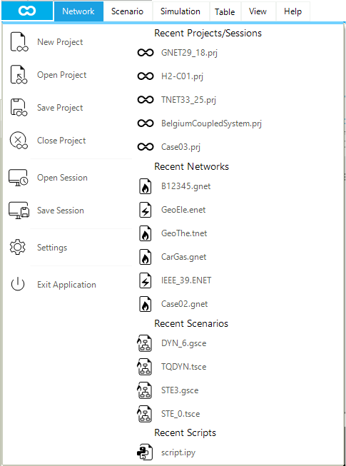
The application menu is accessible from the button at the top-left corner of the GUI. It is divided into two columns, as shown in Figure 3. The first column contains all the project and session-related options, including access to the GUI settings and file version converter. The second column allows the user to access the recent projects, sessions, networks, scenarios, and IronPython scripts.
A project file represents a hierarchical collection of models, profile files, sessions, IronPython scripts, and polygons. Profiles, IronPython scripts, and polygons allow to manage specific aspects at the project level. A model is a child object of a project, and it is a collection of a network, scenarios, state files, solution files, profiles, project file, map file, log files, and model-related IronPython scripts. In releases prior to 3.4, SAInt had also vertex files and labels files. These objects have been moved to the map file and the project file. At this level, profiles and scripts allow to manage model-related aspects, compared to project-related aspects. Finally, a session represents a snapshot of a project containing the state of the tabs available in the map window area of the dock panel and the state of the loaded scenarios. A session preserves the opened windows (e.g., chart windows, map view windows, etc.), tables, and scripts active at the time of saving the session. A specific session can be saved and reopened at a later stage. The position and arrangement of the command line window, the log window, the model explorer, and the property editor are not saved in a session.
The application menu options of the first column are described in Table 2.
| Icon | Options | Description |
|---|---|---|
|
New Project |
Create a new project and close the currently opened project. |
|
Open Project |
Open a previously saved project. A project file has the extension |
|
Save Project |
Save the currently opened project to a project file ( |
|
Close Project |
Close the opened project and the associated networks and scenarios. |
|
Open Session |
Open a previously saved session file. A session file has the file extension |
|
Save Session |
Save the current session to a session file ( |
|
Settings |
Open the general settings to be used in the active project. The settings window allows one to select and set up meteorological data provider, legends colors, default charts, units, fonts, and miscellaneous aspects for the GUI and the solver. |
|
Exit Application |
Option to exit SAInt. If unsaved changes are pending, the user is asked to save the opened model before closing. |


|
Use a session to save a specific time step of interest. |
2.1. Settings
SAInt allows to define a collection of general settings valid for the computer where it is installed. Such settings affect all projects opened or developed on that computer. Model-related settings can be specified in scenarios, default charts, or IronPython scripts. The settings window is designed to centralize the management of all general settings. It contains six tabs: Data Provider, Color Legend, Default Chart, Units, Fonts, and Miscellaneous. Each tab allows addressing specific properties for the default options and settings.
Settings for the units of measure, fonts and the miscellaneous options are saved only when the user clicks on Apply & Exit. If the user cancels or closes the Settings window, the changes are discarded.
The list of options available in the setting are described in Table 3.
| Icon | Options | Description |
|---|---|---|
|
Data provider |
Option to select and set the connection properties for the meteorological data provider. |
|
Plugin |
Option to install or remove plugins. |
|
Color legend |
Option to define branch and node colors and ranges for the legends to be used in the map window. |
|
Default chart |
Option to customize the type and properties of the "default charts" for each object in a model. |
|
Units |
Option to customize currency and reference units of measure for all properties in a model. |
|
Fonts |
Option to customize font family, size, color, and style for the different parts of the GUI. |
|
Default Display Property |
Option to select the properties to display in the node bar. |
|
Miscellaneous |
Option to customize log window, map provider, node bar, polyline properties, and solver-related aspects. |


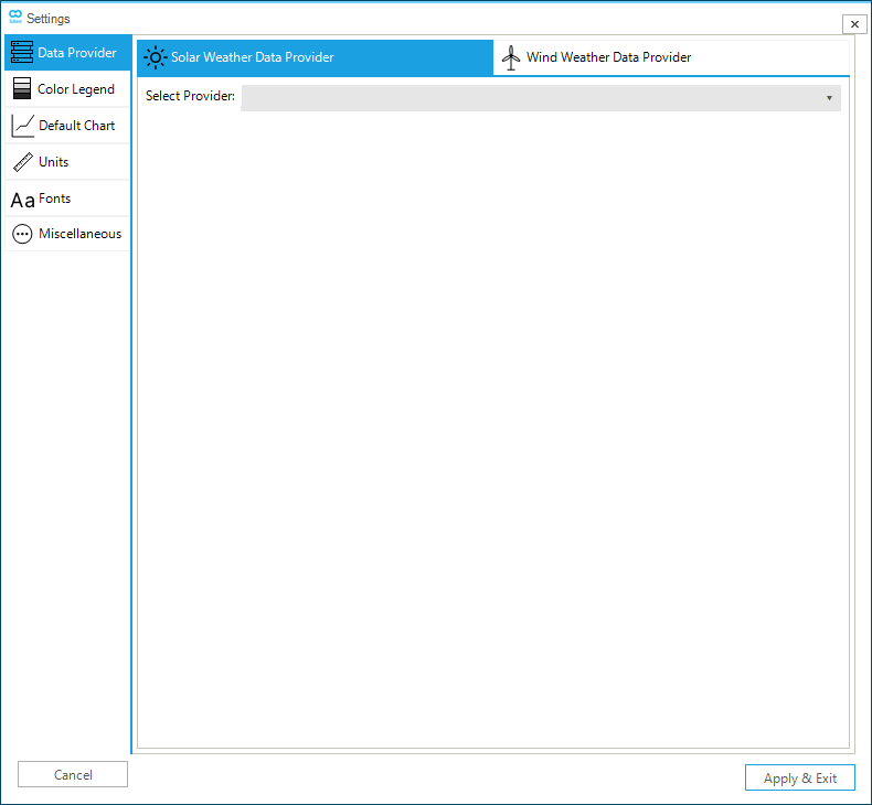
2.1.1. Data provider
The Data provider tab allows the user to select and set the solar and wind weather provider to retrieve data useful to develop an electric network model. For each data provider, the user can specify — if needed — login credentials, server URL, and search criteria (e.g., year, geographic location, time granularity, etc.). Data providers and criteria can be updated or modified at any time by the user. See the section "Integrating Weather Resource Data" for details on the data provider or go to the How-To guide "Connect to Weather Resource Data Providers".
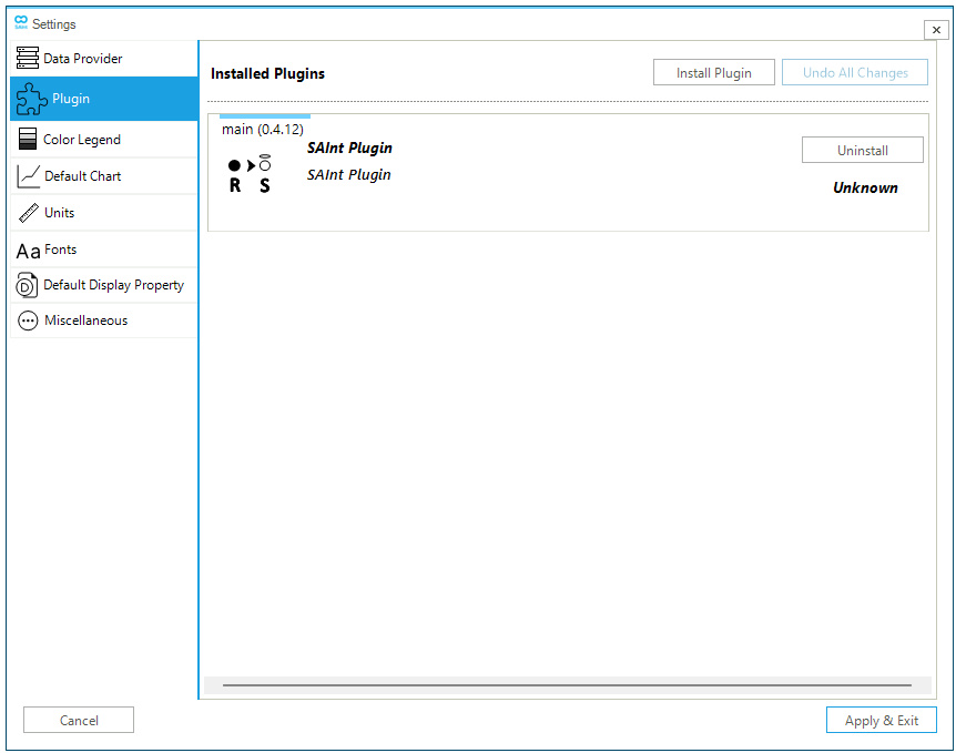
2.1.2. Plugin
The Plugin tab (Figure 5) allows the user to install and remove plugins. During the installation, SAInt checks if the plugin is signed or not, and informs the user. If a plugin is signed by encoord, a blue text stating "Verified" is available below the button Uninstall. An unsigned plugin has the text "Unknown". A progress bar indicates the status of the installation process. If the plugin has its own icon, that will be used, in place of the default plugin icon, in the "Installed Plugin" tab of the general settings and in the tab "Tools" of SAInt’s main windows.
Plugins are removed only after the Apply & Exit is selected.
See the the How-To guide "Install and Execute a Plugin".
|
File-hosting services, like Microsoft OneDrive or Google Drive, may cause problems with plugin reinstallation in SAInt. If, after repeating the installation procedure, the plugin is not available in the Tools tab or in the "Plugin" section of the general settings. Or, if you get an error message indicating that the user does not have write access to the specified installation path. In both cases, you have the As a primary measure to address such problems, we advise excluding the |
|
When installing a plugin, SAInt unpacks the content of the "*.plugin" file in a temporary folder, and after, moves the content of the temporary folder to the It is possible that the security and antivirus software on your machine scans the content of such a temporary folder and blocks its files until any security threats are addressed. This prevents access, copying, or deletion of the plugin’s files. And prevents SAINT from completing the installation. If you get an error message stating that the "Plugin installation failed: Access to the path … is denied." after clicking on Apply & Exit, please repeat the installation and wait some time before clicking on Apply & Exit to allow your security software to finish processing the plugin’s files and release them to be moved. |
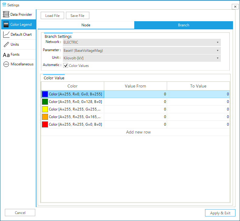
2.1.3. Color legend
The Color legend tab allows the user to edit and customize the legends used to display branches and nodes properties in the map window.
In the case of branches, Figure 6 shows how the legend can be customized per network, parameter, and unit of measure. The options Color, Value From, and To Value allow to obtain a categorized legend, where each class is defined in terms of the range of the values of the parameter, and color. The number of classes can be changed using the option "Add new row". In the example of the figure, the base voltage magnitude, in kilovolts at the branch level, is categorized into 5 classes. Ranges for each class are automatically define as the option Automatic is checked (by default). The blue class starts at minimum value. The red class ends at the maximum value. The remaining breaks are defined by calculating four equally spaced intervals.
The user can customize the following options of the branch legend settings:
- Network
-
Option to specify which type of network to customize (i.e., available values are gas, electric, and hubs, while liquid and heat networks will be available in future releases).
- Parameter
-
Option to select a specific parameter from a drop-down menu based on the selected network type.
- Unit
-
Option to select the unit of measure from the drop-down menu for the specified parameter.
- Automatic
-
Option to let SAInt automatically assigns the color range to the parameter. Untick the option to enforce the user-specified categories.
- Color Value
-
The user can customize color and class range. The
Colorcolumn defines the RGB of the parameter that applies for the intervalValue From—To Value. In addition, new ranges can be added using the Add new row. The color dialog window (Figure 6) is accessible via … located on the right side of theColorcell.
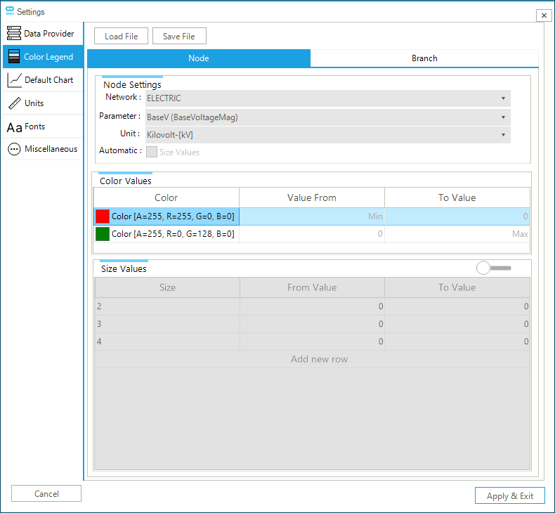
In the case of nodes, Figure 7 shows how the legend can be customized per network, parameter, and unit of measure. The fill color of the nodes can be personalized for results divided into the negative region (i.e., the minimum value and zero excluded), and the positive region (from zero excluded to the maximum). Values equal to zero are represented in a white. If both extreme are in the same region, only one color is visible. The size of the nodes is personalized using a user defined number of classes with their own ranges. The number of classes can be changed. In the example of the figure, only the color is active. No sizing of the nodes is selected as the sliding bar on the right of the "Size Values" entry is not active.
As in the case of the branch legend, the user can customize the following options of the node legend settings:
- Network
-
Option to specify which type of network to customize (i.e., available values are gas, electric, and hubs, while liquid and heat networks will be available in future releases).
- Parameter
-
Option to select a specific parameter from a drop-down menu based on the selected network type.
- Unit
-
Option to select the unit of measure from the drop-down menu for the specified parameter.
- Automatic
-
Option to let SAInt automatically assigns the color range to the parameter. Untick the option to enforce the user-specified categories.
- Color Value
-
The user can customize color and class range. The
Colorcolumn defines the RGB of the parameter that applies for the intervalValue From—To Value. - Size Values
-
The user can specify the number of classes for the different sizes and the range of valid values for each class with the interval
Value From—To Value.
|
SAInt uses a reference colors palette which can be modified by the user at any time. Reference colors are (in RGB format) black (r0g0b0), white (r255g255b255), and red (r255g0b0), plus a series of custom options: r0g157b209, r204g185b116, r140g140b140, r218g139b195, r147g120b96, r129g114b179,r196g78b82, r85g168b104, r221g132b82, and r0g85b137. |
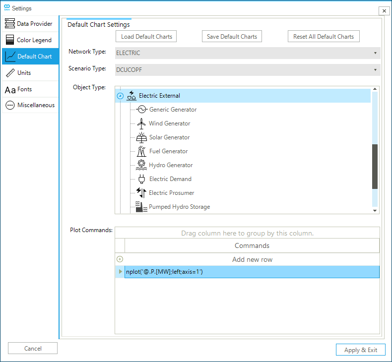
2.1.4. Default chart
The Default Chart tab allows the user to customize the "default charts" produced by SAInt for the different network objects. Figure 8 shows an example of electric externals in a DCUCOPF scenario of an electric network. Please, note that only a parent object can be customized in terms of properties, units, axis, color, and so on in the chart. A child object inherits the graphical properties from its parent object, and so its own chart’s properties cannot be modified. A customized default charts configuration file can be saved for future use or loaded from a previous project. After customization, the user can also reset all specified properties to the installation defaults. The plot commands section displays the function used to generate the default plot.
The user can select the following options of the default chart settings:
- Load default charts
-
Option to load a saved default chart file with
*.dfcextension. - Save default charts
-
Option to save the customized default chart configuration to a file with
*.dfcextension. - Reset all default charts
-
Option to reset all plots to the SAINt installation default configuration.
- Network type
-
Option to specify which type of network to customize (i.e., available values are gas, electric, and thermal).
- Scenario type
-
Option to filter the type of objects to customize based on the selected scenario type available from the drop-down menu.
- Object type
-
The option lists, in a hierarchical tree form, the parent and child objects based on the network and scenario selected.
- Plot commands
-
Option to edit the script for the default plot of the specified parent object.
|
Default charts are displayed when selecting from the objects' context menu. |
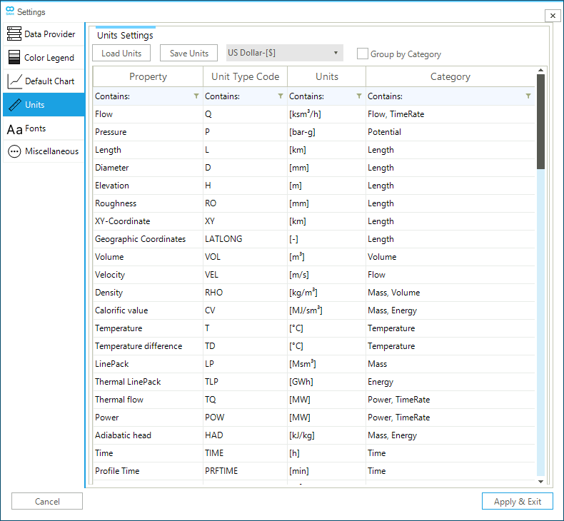
2.1.5. Units
The Units tab allows the user to specify the currency and the units of measure for all properties of parameters and quantities estimated in SAInt. As shown in the example of Figure 9, objects' properties are listed along with their SAInt code, and the unit of measure, which is accessible from a drop-down list ▼. Properties can be grouped to facilitate management operations. The settings can be saved to an external units file, or loaded from an external units file. SAInt centralizes the management of units of measure in the units tab, but it allows to use of alternative units in charts or simulation scenarios, and it takes care of a correct units conversion. For a step-by-step explanation of the use of the unit settings go to the How-To guide "Change Units of Measure and Currency".
Once the units of measure are set, they are valid for all projects, till the next change. Unit settings are a property of the software installation and not of a SAInt project or model. The user should pay attention when moving a project from one computer to another, because the local machine settings for the units may be different, and SAInt will automatically perform all necessary conversions.
The user can select the following options from the units settings:
- Load units
-
Option to load a saved units configuration file with
*.unitsextension. - Save units
-
Option to save specific units settings to a file with
*.unitsextension. - Group by category
-
Option to group properties by category.
- Currency change
-
The user can set a currency value in the GUI by choosing from the list of currencies (i.e., US dollar, British Pound, and Euro). The default value is US dollar.
- Units
-
The user can select from a drop-down menu a specific unit of measure for each one of the available properties.
Templates for the most common settings for the units of measure complying with the International System and the Imperial system are available in the directory Units under .\encoord\SAInt-v3\Settings.
|
When creating a new project, it is recommended to define a custom unit configuration or to select one of the predefined configurations available in |
2.1.6. Fonts
The Fonts tab allows to personalize font properties for all parts of the GUI. As showed in Figure 10, the user can change fonts in the Command Window, the Map Window, the Log Window, the Project and Model Explorer, Workspace, tables, charts, and globally.
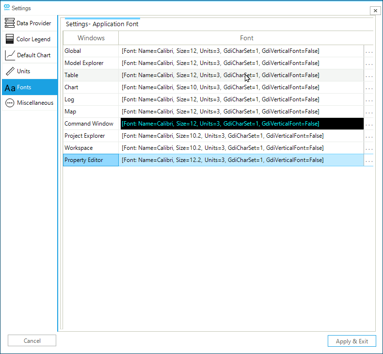
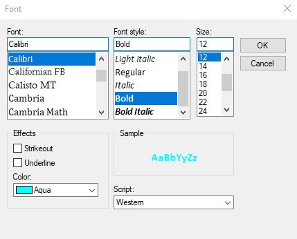
The font dialog box is accessible via … on the right side of the font column. The dialog box allows customizing the font family, the font style, the font size, effects, color, and script. A preview is shown in the sample section. The font color is used only to modify the Command Window.
2.1.7. Default Display Property
The default display property tab allows selecting which properties should be displayed in the node explorer (Figure 12) which facilitates navigation of your model and results by exploring nodes.
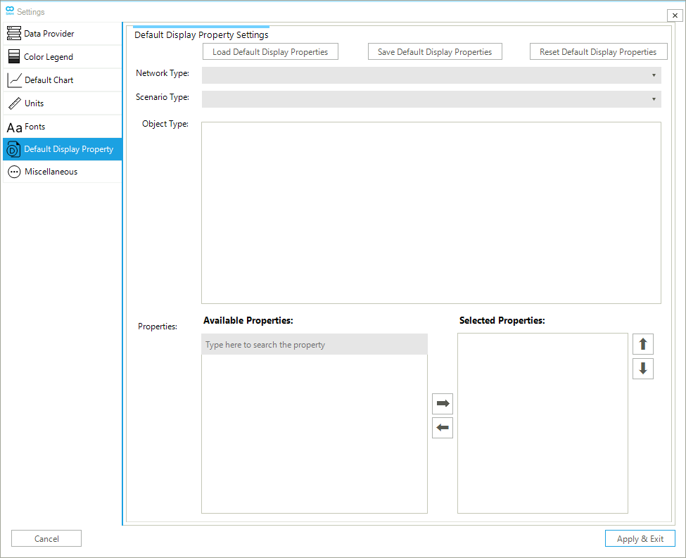
The default display property tab is like the default chart tab as they share the same object selection method as well as load, save, or reset options. The user can modify the following options of the display property tab:
- Load default display property
-
Option to load a saved default property file with a
*.ddpextension. - Save default display property
-
Option to save the customized default display property configuration to a file with a
*.ddpextension. - Reset default display property
-
Option to reset the list of the displayed properties to the SAInt installation default configuration.
- Network type
-
Option to specify which type of network to customize (i.e., available values are gas, electric, and thermal).
- Scenario type
-
Option to filter the type of objects to customize based on the selected scenario type available from the drop-down menu.
- Object type
-
The option lists, in a hierarchical tree form, the parent and child objects based on the network and scenario selected.
- Available property
-
The option lists all the available properties for the selected object. The list may change depending on whether an active scenario or a valid loaded solution is available.
- Selected property
-
List of the user-selected properties to be displayed in the node bar. The entries are selected from the "Available Properties" lists. The list can be expanded or reduced by moving entries between the "Selected Properties" box and the "Available Properties" box using the two buttons with left- and right-pointing arrows.
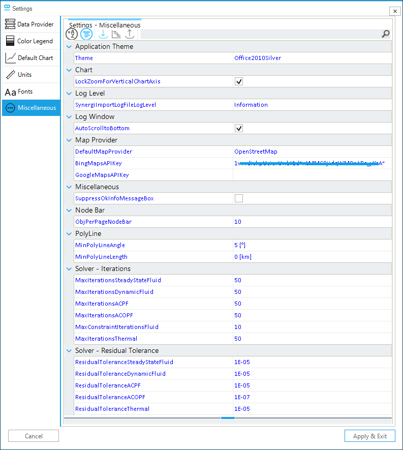
2.1.8. Miscellaneous
The miscellaneous tab allows editing the properties related to GUI, imported polylines from a shapefile, solver iterations, solver residual tolerance, and other properties, as shown in Figure 13.
The user can modify the following options of the miscellaneous tab:
- Theme
-
Change the look and feel of the GUI by applying different application themes.
- LockZoomForVerticalChartAxis
-
Lock the zoom on the vertical axis in newly created charts.
- DateTimeFormat
-
Option to select the format of date and time used by SAInt in tables, charts and for importing or exporting time-related data. By default, the first time SAInt is installed, it tries to use the operating system’s user-defined format for the region selected under "" in Microsoft Windows©. (i.e., SAInt combines the format for "Short date" and for "Short time" used in your machine). The user can change this format in SAInt-GUI and in SAInt-API, and select among one of the accepted variants. Valid options are:
yyyy-MM-dd HH:mm,yyyy/MM/dd HH:mm,dd-MM-yyyy HH:mm,dd/MM/yyyy HH:mm,MM-dd-yyyy HH:mm,MM/dd/yyyy HH:mm, or the reserved wordsystemwhich bring the short date and time of the system (in the API). The symbols indicate:MMis the month,ddis the day,yyyyis the year,HHis the hour, andmmare the minutes.Note that the selected format is valid only for work sessions in SAInt-GUI and have no impact on the SAInt-API side, or the other way round, a change via the API does not affect the GUI.
- SynergiImportLogFileLogLevel
-
Option to set the minimum log level for the Synergi import log file by using the ▼ button. Possible log levels, from the more to the less detailed, are verbose, debug, information, warning, error, and fatal. The default value is "Information".
- ThreePhaseConnectivityCheckLogLevel
-
Option to set the minimum log level for the three-phase connectivity check log file by using the ▼ button. Possible log levels, from the more to the less detailed, are "debug", "information", and "warning". The default value is "Debug".
Warning: Only critical connectivity issues that may cause an error when running the simulation are logged.
Information: Additional information about the connectivity checking process and critical connectivity issues is logged.
Debug: Information about the connectivity checking process and details of critical and non-critical connectivity issues are logged.
- AutoScrolltoBottom
-
Option to activate or deactivate the auto-scroll to the bottom of the log window when a new row is added.
- DefaultMapProvider
-
Option to select the default map provider to use in the Map Window for the base map. A drop-down list provides the valid options. The user can specify a different provider for each map view using the Base Map Layer Settings" of the layer window, and must save a session to be able to restore the choice.
BingMapsAPIKey: Insert the user’s API key for the Bing Maps provider. Provided for legacy user of the "Bing Maps for Enterprise service", which will be retired by Microsoft by June 30th, 2028.
GoogleMapsAPIKey: Insert the user’s API key for the Google Maps provider.
AzureMapsAPIKey: Insert the user’s API key for the Azure Maps provider by Microsoft.
- SuppressOkInfoMessageBox
-
Option to show or not informative boxes that require the user to only press Ok.
- MinPolyLineAngle
-
Option to set the minimum deflection angle between two neighboring vertices of a segment of a polyline geometry to identify vertices to remove for reducing and simplifying the complexity of a polyline. IF the angle between the first and second vertex is smaller than the threshold and the
MinPolyLineLengthis smaller, the vertex is removed. - MinPolyLineLength
-
Option to set the minimum allowed perpendicular distance (in liner units, generally meters) before removing a vertex using the "Ramer-Douglas-Peucker algorithm". The basic algorithm is extended by incorporating also an angular criterion (defined by the parameter
MinPolyLineAngle) and and hard-coded static length-excess threshold for keeping vertices in shallow curves (i.e., a fixed value of 1000 meters for geographic data or 10 meters for Cartesian data). - MaxResidualIterationsSteadyStateFluid
-
Option to set the default maximum number of iteration steps used for new steady state scenarios for fluid networks.
- MaxResidualIterationsDynamicFluid
-
Option to set the default maximum number of iteration steps used for new dynamic scenarios for fluid networks.
- MaxResidualIterations(U)ACPF
-
Option to set the default maximum number of iteration steps used for new (unbalanced) AC-power flow scenarios.
- MaxResidualIterationsACOPF
-
Option to set the default maximum number of iteration steps used for new AC-optimal power flow scenarios.
- MaxControlIterations
-
Option to set the default maximum number of constraint and control handling iterations steps used for new steady state and (quasi-)dynamic scenarios
- MaxResidualIterationsThermal
-
Option to set the default maximum number of iteration steps used for new thermal scenarios.
- ResidualToleranceSteadyStateFluid
-
Option to set the default residual tolerance used for new steady state scenarios for fluid networks.
- ResidualToleranceDynamicFluid
-
Option to set the default residual tolerance used for new dynamic scenarios for fluid networks.
- ResidualToleranceACPF
-
Option to set the default residual tolerance used for new AC-power flow scenarios.
- ResidualToleranceACOPF
-
Option to set the default residual tolerance used for new AC-optimal power flow scenarios.
- ResidualToleranceThermal
-
Option to set the default residual tolerance used for new thermal scenarios.
|
SAInt’s default date and time format is |
|
In an Excel™ scenario import file, the property |
3. Ribbon tabs
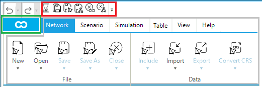
The Ribbon tabs part of the ribbon bar consists of six tabs (Figure 14 top): network, scenario, simulation, table, view, and help. Each tab is composed of several panels (e.g., for the Network tab we have the panel File and Data). Each panel contains different menu items or options (e.g., the Data panel of the Network tab has the following options: New, Open, Save, Save As, and Close). By using the button ▼ in each option, the user can open a drop-down containing different specific functions. The ribbon tab can be minimized by using the  option.
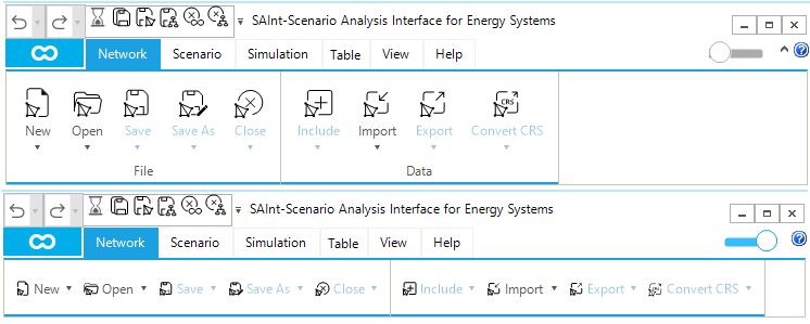 for changing the ribbon tabs part from and to the expanded and minimized version. The ribbon tabs part has six tabs, with multiple panels and options.
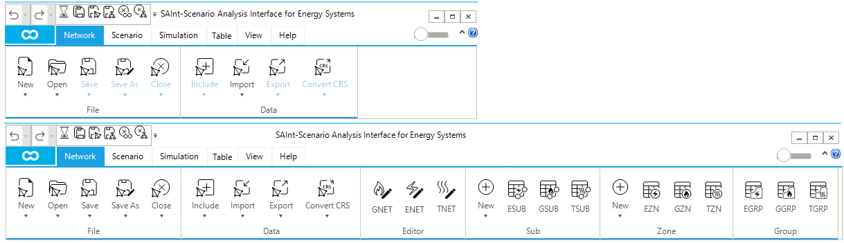
3.1. Network tab
The Network tab of the ribbon bar allows the user to access an extended set of network-related functions. It is composed of up to six panels, depending on the number and type of networks loaded. (Figure 15) shows the case of a project where there is no loaded network (the top part with the two panels File and Data), and the case of a project where a hub, an electric, and a gas network are loaded (the bottom part with six panels: File, Data, Editor, Sub, Zone, and Group). A detailed description of the panels and the available options is provided in the following sections of the reference guide.
3.1.1. File panel
The File panel of the Network tab allows the user to create, open, save, copy, and close any network file available in the active project. Table 4 describes in detail the options available in the File panel.
| Icon | Options | Description |
|---|---|---|
|
New |
Option to create a new prototype network with default property values. The network is a placeholder for the user’s data. From the drop-down menu ▼ the user can select the type of network (i.e., a gas network, an electric network, or a hub system) and if the type of coordinate type (i.e., Cartesian system or geographci system). |
|
Open |
Option to open a saved SAInt network or Hub system. Use the drop-down menu ▼ to select the type of network. |
|
Save |
Option to save a network to a |
|
Save Copy |
Option to save a copy of an existing network letting with a different name. |
|
Close |
Option to close the active network. |


|
To quickly make a copy of a network, use the button Save As. |
|
When opening a model created prior to SAInt 3.5, a backup copy of the model and the data are created in the folder |
3.1.2. Data panel
The Data panel of the Network tab allows to import and export of data from and to SAInt. The user can include available data in SAInt format in the loaded network, import external data in different formats, or export SAInt data and networks to native or exchange formats. Table 5 describes in detail the options available in the Data panel.
| Icon | Options | Description |
|---|---|---|
|
Include |
Option to include native SAInt data files related to the type of network ( |
|
Import |
Option to import external data files related to the type of network active in the project (e.g., network, parameter, etc.). |
|
Export |
Option to export data files in SAInt native or exchange formats related to the type of network active in the project. |
|
Convert CRS |
Option to convert the network data CRS to SAInt default geographic CRS to disply a network on a base map. |


The "include" option is designed so that the user can append or incorporate data, already in SAInt native format, in the active project. The data don’t need any transformation and are immediately available. Include allows to:
- Network file
-
Option to include an "existing network" in SAINt native format.
- Polygon file
-
Option to include a "existing polygon file" in the active network.
- Wind turbine power curve file
-
Option to include a existing WTPC file in the active network.
- Fuel consumption curve file
-
Option to include a existing FCC file in the active network.
The "import" option is designed so that the user can transfer data into the active project from an external data source. The data need to be properly prepared and transformed. Templates are provided to support the user in the preparation phase and to reduce possible sources of errors. Import allows to:
- Network
-
Option to import a network using available "network templates". If the coordinate reference system of the data is specified, SAInt will automatically convert the system (CRS) to SAInt’s default CRS (i.e., WGS84 or EPSG:4326) and display the network on a base map.
- From Parameter Import File
-
Option to import parameters' values from an external source using the "parameter import files" to update a network.
- Wind turbine power curve
-
Option to import an external WTPC using a "WTPC template file".
- Fuel consumption curve
-
Option to import a "existing FCC file" in the active network.
- Gas quality
-
Option to import external data on gas quality using the "gas quality template file".
- Synergi
-
Option to import a Synergi file with
.mdbextension and to convert it into a SAInt gas network file with .gnet extension. - Shapefile > Network
-
Option to import network data from an external source in "shapefile format".
- Shapefile > Polygons
-
Option to import polygons data from an external source in "shapefile format".
The Export option is designed so that the user can transfer data from SAint to other SAInt users in a native format or to other users if an external format. SAInt uses the same templates or formats used for importing or including data. Export allows to:
- To Network Import File
-
Option to export network data to a "network import file". If the coordinates of the active network are base on SAInt’s default CRS (i.e., the network is displayed on a base map in the Map View window), the user can export the network to a different CRS. Figure 16
- Wind Turbine Power Curve
-
Option to export the WTPC included in an electric network to a "WTPC file".
- Fuel Consumption Curve
-
Option to export the FCC included in an electric network to a "FCC file".
- To Gas Quality Import File
-
Option to export gas qualities to a "gas quality import file".
- To Parameter Import File
-
Option to export all the parameters of the network to a "network parameter import file".
The "convert" option is designed so that the user can convert the coordinate reference system (CRS) of the active network in a Cartesian map view to SAInt’s default CRS. The conversion procedure opens the network on a new geographic map view and closes the Cartesian one.
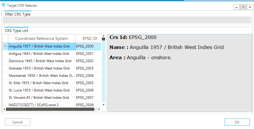
By selecting Convert CRS the user can choose among the available active networks. Figure 17 shows the window where the user can choose the CRS of the active network (i.e., the CRS of the displayed network in the Cartesian map view). The coordinates will be transformed to the CRS EPSG:4326 (i.e., WGS84). The user can select the desired CRS from the available list or filter and select by entering a string or the EPSG code in the "Filter CRS Type" field.

|
Sections "Coordinate Reference Systems" and "Map view" provide more details on how SAInt handles coordinates and coordinate reference systems. |
3.1.3. Editor panel
The "editor panel" of the Network tab gives access to the property editor for the networks available in a project in the GUI. The network property editor contains input and output properties such as the number of nodes, type of network, etc. The available items in the editor panel depend on the type of networks in the active project (e.g., the *.gnet editor is not visible if no gas network is loaded). Table 6 describes in detail the options available in the editor panel.
| Icon | Options | Description |
|---|---|---|
|
ENET |
Option to open an electric network editor. |
|
GNET |
Option to open a gas network editor. |
|
TNET |
Option to open a thermal network editor. |
|
HUBS |
Option to open a hub system editor. |


3.1.4. "Sub" panel
The "Sub" panel of the network tab allows the user to create new sub-system in any network of the active project in the GUI, or to open a table in the dock panel describing sub-systems. The available items in the "Sub" panel depends of the type of networks in the active project (e.g., the *.GSUB table is not visible if no gas network is loaded). Table 7 describes in detail the options available in the "Sub" panel.
| Icon | Options | Description |
|---|---|---|
|
New |
Option to create new subs based on different options. |
|
ESUB |
Option to open a table with a list of electric subs. |
|
GSUB |
Option to open a table with a list of gas subs. |
|
TSUB |
Option to open a table with a list of thermal subs. |


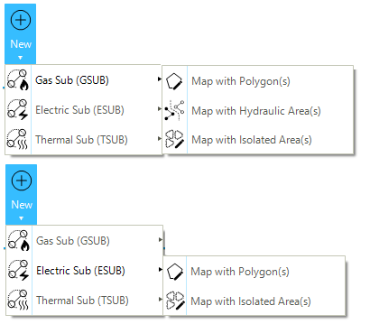
The "New" option is designed so that the user can create a new sub-system in a network by using polygons or properties of the network (Figure 18). The New option allows the user to:
- Map with polygon(s)
-
Create a new sub-system based on polygon(s) included in the network.
- Map with hydraulic area(s)
-
Create a new sub-system based on the hydraulic area(s) of the active gas network. This option is available only for gas and thermal networks.
- Map with isolated area(s)
-
Create a new sub-system based on the isolated area(s) of the active network.
|
The option "Map with polygon(s)" is available only for Cartesian networks, not geographic ones. |
|
When using the "Map with …" functions, the existing subs are deleted and replaced by new ones. The user may need to revise the names of the new subs. |
3.1.5. Zone panel
The Zone panel of the Network tab allows the user accessing tables with a list of zones and their corresponding properties. The type of options shown in the panel depends on the type of networks in the active project (e.g., a *.GZN table is not visible if no gas network is loaded). Table 8 describes in detail the options available in the Zone panel.
As in the case of "subs", the "New" option allows the user to create a new zone using polygons, hydraulic areas (for gas and thermal networks), or isolated areas. When using the mapping functions, the existing zones are deleted.
| Icon | Options | Description |
|---|---|---|
|
New |
Option to create a new zone. |
|
EZN |
Option to open the table with a list of electric network zones. |
|
GZN |
Option to open the table with a list of gas network zones. |
|
TZN |
Option to open the table with a list of thermal network zones. |


3.1.6. Group panel
The Group panel of the Network tab allows the user accessing tables with a list of groups and their corresponding properties. The type of options shown in the panel depends on the type of networks in the active project (e.g., a *.EGRP table is not visible if no electric network is loaded). Table 9 describes in detail the options available in the Group panel.
| Icon | Options | Description |
|---|---|---|
|
EGRP |
Option to open a table with a list of electric network groups. |
|
GGRP |
Option to open a table with a list of gas network groups. |
|
TGRP |
Option to open a table with a list of thermal network groups. |


|
The property editor for a sub, zone, and group can be accessed by using the button Open Editor from their context menu available in the table or model explorer. |
3.1.7. Change Tracking
The Change Tracking panel of the Network tab allows the user to access and manage the tracking functionality for changes in networks and objects in SAInt. This is not an "undo" option and does not allow for automatic rolling back or forwarding of changes. But it is a logging tool to record changes implemented in a network model, like adding or removing objects, or modifying the properties of one or multiple objects. Track Changes does not cover changes to events or scenarios, and it does not monitor labels, geographic properties of nodes and branches (e.g., coordinates of nodes and vertices, length of branches), graphical properties of nodes and branches (accessible from the context menu in the Layers Window), or gas qualities and components in gas models.
Table 10 describes the options available in the Change Tracking panel. Logging of changes is available by default when one network is loaded in the active project. But it can be turned off using the "Deactivate" option corresponding to pulling down the blue lever next to the Track Changes icon. Deactivating means that any later change is not recorded, and only by reactivating does the monitoring start again. The data logged for any change is organized and presented to the user in a "Change Tracking Log" table. The user can open the table using the "Show Changes" icon.
Changes are logged every time the option is active, and the user performs an editing action on objects or properties. However, changes are permanently saved only when the modified network is saved, and a track changes file is created for each network in the project. This implies that any unsaved network will not only lose any possible changes, but also that these changes will not be recorded in the track changes log file. The track changes table will report any unsaved in-memory changes, but does not save such changes if the network is not saved. The log file is saved in the same folder as the modified network with file name "type of network . network name . chg". For example, changes to a gas network named Test are saved in the track changes log file named "GNET.Test.chg". After its creation, the changes log can be retrieved and visualized with the "Show Changes" option.
| Icon | Options | Description |
|---|---|---|
|
Show Changes |
Option to open a table with a list of recorded changes. |
|
Activate / Deactivate |
Option to activate or deactivate the tracking of changes to networks or other objects. |

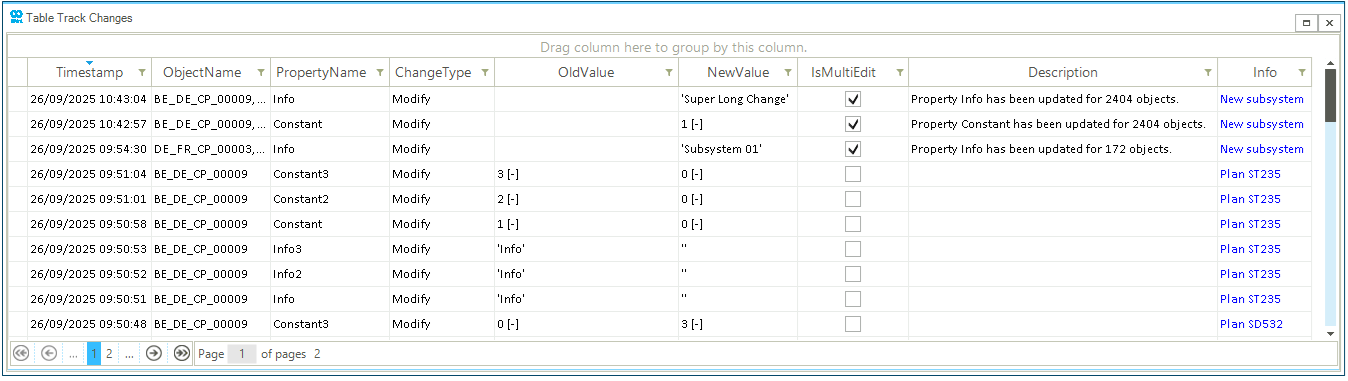
For each change, the following attributes are logged and accessible in a dedicated table (see Figure 19 for an example):
- TimeStamp
-
it records the "timestamp" — i.e., the date and time — of when a change is taking place. The column is visible by default.
- Network
-
it records the name of the network where the change takes place. This is particularly useful when the project has more than one network. The column is hidden by default. Use the Column Chooser to add it to the table.
- ObjectName
-
it reports the name of the object where the change takes place. In case of a multi-edit operation, the list of all objects modified is provided. The list of objects can be very long. Hovering over the cell opens a new window displaying the list of objects and the option to copy and paste to an external editor to retrieve the full list. The column is visible by default.
- PropertyName
-
it is the name of the property modified by the change. The column is visible by default.
- ChangeType
-
type of change is recorded in one of three categories: "Add" when a new object is added to the model, "Remove" when an object to deleted from the model, and "Modify" when a property is changed for one or more objects. The column is visible by default.
- OldValue
-
it is the value of the property for an object before the change. The column is visible by default.
- NewValue
-
it is the new value assigned to the changed object property by the user. The column is visible by default.
- IsMultiEdit
-
the attribute reports with a true or false value if the change is modifying a single object or multiple objects at the same time using the multi-edit functionality of SAInt. The properties and the number of objects modified is reported in the attribute "Description" for any instance of "IsMultiEdit" equal to true. The "ObjectName" attribute reports the complete list of names of objects changed. The column is visible by default.
- UserName
-
it is the name of the user of the operating system who has logged in and launched SAInt to work on a model or project. This attribute may be relevant when multiple users are working on the same model. The column is hidden by default. Use the Column Chooser to add it to the table.
- Description
-
a short message describing which properties have been changed and for how many objects. This attribute is populated only for multi-edit changes. The column is visible by default.
- Info
-
it provides an editable field to record user-specified details for the change. It is the only editable field in the Track Changes table. The column is visible by default. Multi-edit is available after selecting two or more rows in the table and accessing the context menu by right-clicking.
As with any other table in SAInt, the table of Track Changes can be filtered, searched, sorted, and exported outside SAInt. Check the context menu of the table for available options. The user can adjust which attributes to list in the table, modify the columns' width, and group rows based on column’s values. Cell or row content can be copied and pasted (using CTRL+C and CTRL+V) once selected (i.e., highlighted in blue). The table shows a maximum of 50 rows per page. The user can find the table navigation options at the bottom of the window. The options cover back and forth arrows, page selection and page number selection.
|
Multi-edit changes are recorded as an aggregated change. They are reported as a single row in the table of Track Changes, and are clearly identified by the property of the attribute "IsMultiEdit" and the presence of a value in the "Description" attribute. It is not possible to explore any change for a single object or a subset of the initial group of objects. |
|
The table can be exported to an external file in Excel, CSV, PDF, or HTML format. When using the Excel format, a multi-edit change can record a string of text longer than Excel’s supported maximum length. This will not prevent the file from being created, but Excel will require the user to perform a "recovery" operation to open the file. The CSV or HTML formats are better options when complex multi-edit changes are present. |
3.2. Scenario tab
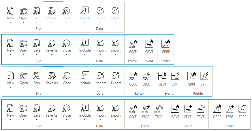
The Scenario tab of the ribbon bar allows the user to access an extended set of scenario-related functions. It is composed of up to five panels, depending on if a scenario is active and on the type of scenario in the project. (Figure 20) shows the case of a project where there is no scenario active (the top part with the two panels File and Data), a case of a scenario for a dynamic gas model (second from top with the five panels File, Data, Editor, Event, and Profile), a case of a scenario for a dynamic gas and quasi-dynamic electric coupled models (third from top), and a case with (quasi-)dynamic gas, electric and thermal models. A detailed description of the panels and the available options is provided in the following sections of the reference guide.
3.2.1. File panel
The File panel of the Scenario tab, similarly to the File panel of the Network tab, allows the user to create, open, save, copy, and close any scenario file available in the active project. Table 11 describes in detail the options available in the File panel.
| Icon | Options | Description |
|---|---|---|
|
New |
Option to create a new scenario for the active network using a dedicated Scenario Dialog window. |
|
Open |
Option to open an existing scenario for the active network. The user can select the scenario from the ones available in the Scenario Dialog window. |
|
Save |
Option to save the current scenario for the active network. |
|
Save As |
Option to save and copies the current scenario letting the user changing its name. |
|
Close |
Option to close the current scenario for the active network. |


3.2.2. Dialog window
The Dialog window of the Scenario tab allows the user to define all necessary scenario properties or to select an existing scenario from the ones available in the active project. Figure 21 shows an example of a Scenario Dialog window for an electric DCUCOPF scenario (top) and an example of the scenario properties section for a dynamic gas scenario (bottom). In the example of the electric DCUCOPF scenario, it is possible to see that a SteadyACPF scenario has been already created, and it is available in the scenario list section. The scenario properties change according to the scenario type.
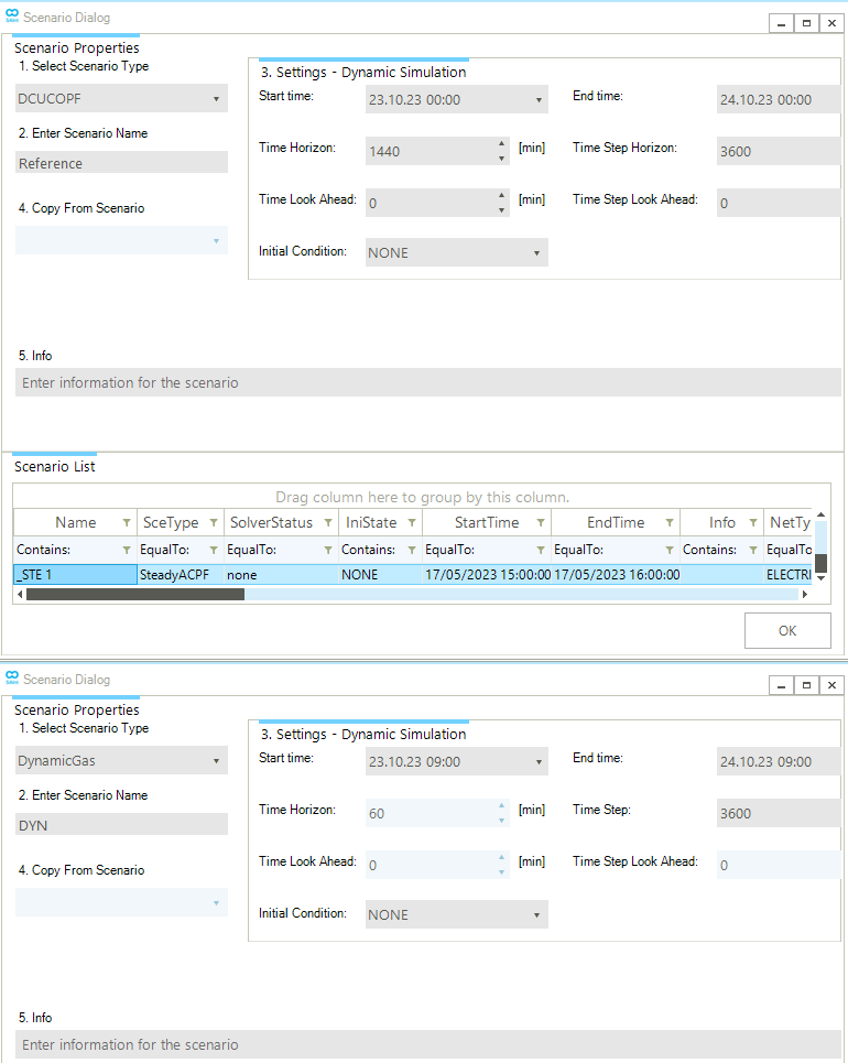
The Scenario Dialog window is designed so that the user can define or review the main properties of a simulation scenario. The list of options is the following:
- Select scenario type
-
Option to select the scenario type among the available type for the chosen network (e.g., DCUCOPF, SteadyACPF, DynamicGas, etc.).
- Enter scenario name
-
Option to specify the name of the scenario to load or create.
- Copy from scenario
-
Option to copy a scenario, and transfer the associated events and profiles, to the new scenario. This option is available only when using the button Save As from the File panel.
- Start time
-
Define the start time of the scenario expressed as date and time. Date and time can be selected from a drop-down menu or typed manually with the format dd.mm.yyyy hh:mm (e.g., based on the format day.month.year hours:minutes like in the case 21.01.1973 18:30 which is January 21 1973 at half past six in the afternoon).
- End time
-
Option to define the end time of the scenario expressed as date and time. The date and time can be selected from a drop-down menu or typed manually.
- Time horizon
-
The time horizon is a fraction of the scenario time window considered for an optimization or solution step in dynamic scenarios. It is expressed in seconds. For example, a time horizon of 600 seconds indicates that an optimization or solution step is set for every 10 minutes.
- Time step horizon
-
An integer time step in minutes indicating a fraction of the scenario time window used for discretizing the scenario time window into distinct time points which are calculated for the simulation variables. The option is valid only for DCUCOPF scenarios.
- Time look ahead
-
It is a time duration added to the time interval considered in the consecutive optimization for DCUCOPF scenarios.
- Time step look ahead
-
The "integer time step look ahead" is a fraction of the scenario time look ahead used for discretizing the scenario time look ahead into distinct time points which are calculated for the variables. Valid for DCUCOPF scenarios.
- Initial condition
-
Option to set the initial scenario conditions for a quasi-dynamic or dynamic scenario. It can be the solution to a steady state scenario or the terminal state of a quasi-dynamic or dynamic scenario.
- Info
-
Option to add a comment or description for the scenario.
- Scenario list
-
Option to list all existing scenarios linked to the active network.
|
Before 3.4 release, scenarios had a Comment option instead of Info. However, comments are no longer supported, i.e., the comments will not be mapped to the new Info option. |
3.2.3. Data panel
The Data panel of the Scenario tab contains buttons to include, import, or export scenario events, profile, result, and network state to and from SAInt. The user can include available data in SAInt format in the active model, import external data in different formats, or export SAInt data and scenario-related information to native or exchange formats. When dealing with power flow simulations or DCUCOPF optimization problems, a "Transfer" option is available to export commitment, dispatch or demand events of a solved scenario to be used as input to another scenario. Table 12 describes in detail the options available in the Data panel.
| Icon | Options | Description |
|---|---|---|
|
Include |
Option to include native SAInt data for loading a scenario file ( |
|
Import |
Option to import template files related to the scenario (e.g., event, profile, etc.). |
|
Export |
Option to export data to external files related to the scenario (e.g., to Excel, SAInt native, etc.). |
|
Integrated Planner |
Option to export commitment, dispatch or demand events to a new SAInt scenario or to new import files to perform a "state transfer" from a DCUCOPF or transfer events from a ACPF/UACPF to other electric simulations or optimization problems. This option is only available when an ACPF quasi-dynamic scenario or a DCUCOPF scenario are loaded and solved. |


The Include button provides the following options:
- Scenario event(s)
-
Option to include scenario events from an existing "scenario file" for *.esce, *.gsce, or *.tsce to the current scenario.
- Profile(s)
-
Option to include scenario profiles from an existing "profile file"
*.prflto the current scenario.
The Import button provides the following options:
- Scenario event(s)
-
Option to import scenario event(s) using an "events import file" to the current scenario.
- Profile(s)
-
Option to import profile(s) using an "profile import file" to the current scenario.
The Export button provides the following options:
- Scenario event(s)
-
Option to export the current scenario events to an "events import file".
- Profile(s)
-
Option to export the profiles from the current scenario to a SAInt " profile file" (*.prfl).
- Results
-
Option to export the specified results to a "result output file". The user is required to provide the results description file, which contains a list of properties, and the path to save the exported results.
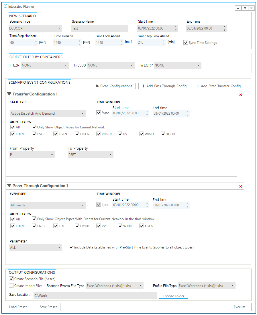
The Integrated Planner button opens the "integrated planner" tool which allows to save commitment, dispatch or demand events from an steady state ACPF simulation, a quasi-dynamic ACPF simulation or a DCUCOPF optimization to create a new scenario to be used as input for other simulations or optimizations. Figure 22 shows an example of the form, while a detailed description of the tool is provided in "Exporting data to a new SAInt scenario file: the Integrated Planner tool".
3.2.4. Editor panel
The Editor panel of the Scenario tab allows the user to access the property editor for the active scenario in the GUI. The user can use the property editor to modify all aspects of a steady state or dynamic scenario such as simulation start and end time, time step, initial state, solver type, look ahead, etc. The type of buttons shown on the panel depends on the type of active network. Table 13 describes in detail the options available in the scenario Editor panel.
| Icon | Options | Description |
|---|---|---|
|
GSCE |
Option to open a gas scenario in the property editor. |
|
ESCE |
Option to open an electric scenario in the property editor. |
|
TSCE |
Option to open a thermal scenario in the property editor. |


3.2.5. Event panel
The Event panel of the Scenario tab allows the suer to access the scenario events table in the GUI. The user can use the table to manage all events of the active scenario. Table 14 describes in detail the options available in the scenario Event panel.
See the How-To guide Create a scenario event in SAInt-GUI for a step-by-step description on managing events.
| Icon | Options | Description |
|---|---|---|
|
GEVT |
Option to open a table with a list of events for the active gas scenario. |
|
EEVT |
Option to open a table with a list of events for the active electric scenario. |
|
TEVT |
Option to open a table with a list of events for the active thermal scenario. |


3.2.6. Profile panel
The Profile panel of the Scenario tab allows the user to access the scenario profiles window in the SAInt-GUI. The user can use the profile window to manage profiles saved in the active network. The type of buttons shown on the panel depends on the type of active networks. Table 15 describes in detail the options available in the Scenario Profile panel.
See the How-To guide "Create a Profile in SAInt-GUI" and the guide "Assign a Profile to an Existing Event" for a step-by-step description on creating and assigning profiles.
| Icon | Options | Description |
|---|---|---|
|
GPRF |
Option to open the table with a list of profiles for the active gas scenario. |
|
EPRF |
Option to open the table with a list of profiles for the active electric scenario. |
|
TPRF |
Option to open the table with a list of profiles for the active thermal scenario. |


3.3. Simulation tab
The Simulation tab of the ribbon bar allows the user to access all simulation-related functions for a given model. This tab is only active when a scenario is loaded. It is composed of four panels (Figure 23) from where the user can launch the execution of a simulation, interact with the solver by pausing, stopping or continuing a simulation, checks logs and use the animation functions for dynamic simulations. A detailed description of the panels and the available options is provided in the following sections of the reference guide.

3.3.1. The Execute panel
The Execute panel of the Simulation tab contains functions for launching the execution of the different types of active scenarios available. The type of available buttons depends on the type of active networks. Table 16 provides details on the options. Please, note that a combined simulation can only be run when the time windows of the scenarios (e.g., electric and gas) have the same start and end time.
| Icon | Options | Description |
|---|---|---|
|
Gas |
Option to execute an active gas scenario. |
|
Electric |
Option to execute an active electric scenario. |
|
Thermal |
Option to execute an active thermal scenario. |
|
Combined |
Option to execute a combined (e.g., electric and gas) scenario. |


|
For DCUCOPF scenarios, the user is asked to confirm any new execution that overwrites an existing solution. This extra check is meant to prevent launching a long optimization run or accidentally overwriting a solution. |
3.3.2. The Solver Interaction panel
The Solver Interaction panel of the Simulation tab allows the user to interact with the solver by pausing, stopping, or continuing a simulation. Table 17 provides details on the available options. When stopped, a simulation cannot be continued anymore. When paused, a simulation or optimization can only be restarted by using the Continue. When paused, the SAInt solver is frozen and cannot commit to another problem. Note that in a paused simulation, the time displayed in the map window indicates the latest timestep solved.
When the user stops a (quasi-)dynamic simulation or an optimization using Stop, SAInt aborts execution and reports the status as "failed". Results computed till the moment of stopping are saved. The remaining period of the simulation or optimization is set to "NA" (not available). Similarly, results computed up to the moment of pausing are saved in memory and can be accessed via tables or charts. It is also possible to pause and export the network state to a "*con" file for the latest computed time step, to be used as the initialization state in other simulations (see the option in the Scenario tab).
Results are correctly saved only if the process is stopped in the SAInt-GUI. Results are not correctly saved if the user aborts the process in the API or by killing the SAInt process from the Task Manager of the operating system.
| Icon | Options | Description |
|---|---|---|
|
Pause |
Option to pause a running simulation at the next possible time step. |
|
Continue |
Option to continue a paused simulation. |
|
Stop |
Option to stop and exit a running simulation at the next possible time step. |


|
The Pause option is very useful to analyze partial results during a simulation and check the evolution of your network. |
3.3.3. Log panel
The Log panel of the Simulation tab allows the user to save the log file to a text file, to clear the information displayed in the window or to show a more detailed log file in the GUI. Table 18 provides details on the available options. Every new simulation automatically deletes the previous log files. Warnings are highlighted in yellow, orange, and red, according to the level of severity. The information related to loading and saving files are visible with a white background. The log file can be used to debug an infeasibility.
| Icon | Options | Description |
|---|---|---|
|
Show log |
Option to open the log window if not available in SAInt-GUI. |
|
Save log |
Option to save the log from the log window to an external text file. |
|
Clear log |
Option to clear the active log presented in the log window. |
|
Extended log |
Option to enrich the active simulation log with a more detailed information on the network objects. |


|
The "extended log" is presented to the user after the execution of a simulation or optimization problem. The file is saved in |
|
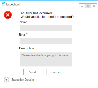
An exception logging mechanism is active when using SAInt API. The mechanism saves the exception log either in the default directory This functionality is available only in the API. |
3.3.4. Animation panel
The Animation panel of the Simulation tab allows the user to navigate through the timesteps of the solved (quasi-)dynamic scenario and see the results in the active map window or charts. Table 19 provides details on the available options. By selecting the shift time using the ▼, the user can visualize inputs or outputs with different time granularity. By pressing Play, the animation starts and repeats until the user clicks again the button to stop it.
When executing a simulation, the user can change the active window to something different from a map. In case a table is selected, an active animation locks the refresh, and the values are not updated dynamically based on the timestep displayed.
The size and color of the arrows in an animation can be changed by modifying the property AnimationArrowSize and ArrowColor in "Branches Layer Setting" of the layer window.
| Icon | Options | Description |
|---|---|---|
|
Slow |
Option to increase the time to display consecutive animation timesteps resulting in a slowdown of the animation. |
|
Play |
Option to start the animation of a solved scenario. |
|
Fast |
Option to decrease the time to display consecutive animation timesteps resulting in a speed up of the animation. |
|
To start |
Option to stop the animation and shifts the animation timestep to the start. |
|
Bwrd |
Option to manually run the animation backwards of a time interval as set in Shift Time. |
|
Shift time |
Option to allow selecting from a drop-down list the animation timesteps to use. The use can select either the time step ( |
|
Frwd |
Option to manually run the animation forward of a time interval as set in Shift Time. |
|
End |
Option to stop the animation and shifts the animation timestep to the end. |


|
When using an animation, all the windows showing results are updated every timestep (defined in the shift time). A red vertical bar appears on the chart window to indicate the timestep. |
3.4. Table tab
The Table tab of the ribbon bar allows the user to access results and properties for all objects (e.g., ENO, GDEM, or HSUP) of the different networks in the active project in tabular form. Figure 24 shows the Table tab in the case of a simulation involving a hub, a gas network, and an electric network. The tab is composed of up to four panels: electric, gas, others, and PLG. The PLG gives access to a table describing the polygons available in the active project. A detailed description of the available options is provided in the following sections of the reference guide.
|
If an animation is running, tables are locked and values are not refreshed. |
|
You can quickly navigate big tables using your mouse’s scroll wheel or your keyboard’s page down / page up buttons to move vertically. You can also use the scroll bars for vertical or horizontal shifting. You can also use your touchpad’s two-finger gestures to move up and down or left and right. |
3.4.1. Table panel by type of network
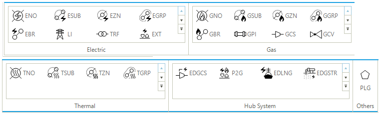
The Electric, Gas, thermal, and Hub System panels of the Table tab allow to access properties and results in tabular form for all network objects in the active project. Use ▼ and ▲ to navigate through the section. Figure 25 shows the expanded form of the three panels after clicking on the drop-down button. By selecting an object in the list, a new table is available in the dock panel of the GUI.
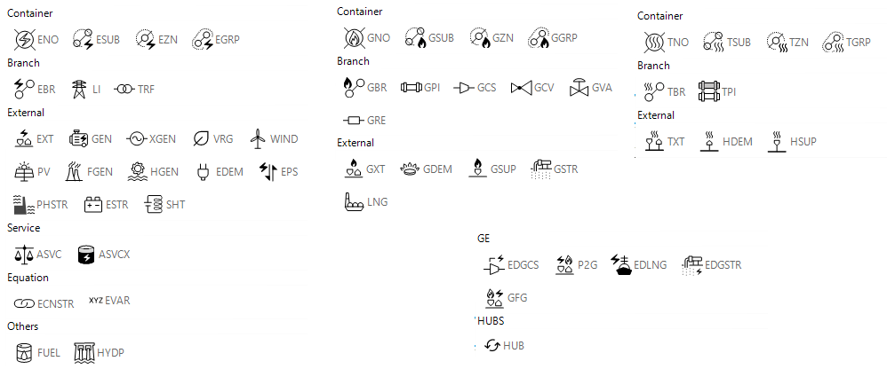
Figure 26 shows, as an example, the result of selecting the FGEN object from the Electric panel. All generators in the active electric network are displayed along with user selected input and output properties. Properties are color coded following this convention:
- Black
-
Read-only properties of an object. These properties are derived (e.g.,
NetType). - Blue
-
Editable network properties of an object. These are input properties (e.g.,
Name). - Red
-
Scenario result properties of an unsolved or failed scenario (e.g.,
P). - Green
-
Scenario result properties of a successfully solved scenario (e.g.,
P).
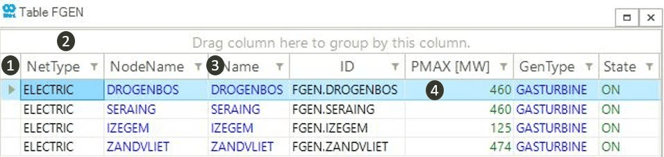
The user can navigate the tabular form of results and properties using three main context menus:
- Global context menu
-
This menu is available by right-clicking at ❶ or ❷ in the generated table (see example of Figure 26). It allows to perform three different sets of tasks: to toggle on or off an extra header and/or tail row in the table for filters, search, or summary tools; to modify, reset and update the available columns in the tables; to export the table to an external file in different formats.
- Column context menu
-
This menu is available by right-clicking on any column name (e.g., right-click at ❸), and it allows the user to add, remove, modify, and style columns in the table.
- Row context menu
-
This menu is available by right-clicking on any cell of a row of the table (e.g., right-click at ❹), and it allows the user to access functions to perform a variety of tasks on the object described by the row. The user can, for example, access the object in the property editor, locate and zoom to it in the map view, and add events to the object.
The options of the global context menu options are shown in Figure 27.
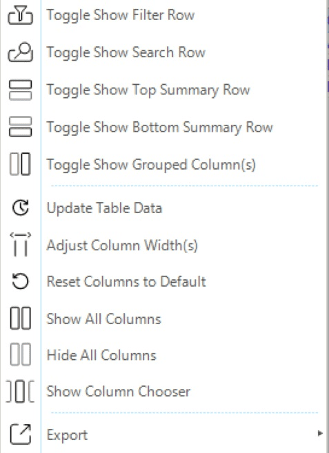
The global context menu allows to:
- Toggle show filter row
-
Option to add or remove a header row to apply filters to select rows based of different criteria like
EqualorContains. - Toggle show top summary row
-
Option to add a summary row at the top of the table. The summary includes the count for string type entries, while the average for float type entries. For float type entries other mathematical operators (like sum, max, etc.) can be chosen by right-clicking on default summary option.
- Toggle show bottom summary row
-
Option to add a summary row at the bottom of columns. The summary options are the same of the top summary row.
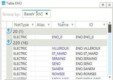
- Toggle show grouped column(s)
-
If the user has grouped table by using a column or multiple column, this options will include add or remove such grouping columns to the table columns. An example is provided in the following figure, which shows how the column BaseV is at the same time available in the table and as a grouping criterion:
- Update table data
-
Option to update and refresh the data of the table based on the current scenario results.
- Adjust column width
-
Option to adjust the width of all the columns to the headers' length.
- Reset columns to default
-
Option to remove all the added toggles.
- Show all columns
-
Option to insert all the possible columns for the current table.
- Hide all columns
-
Option to hide all the columns of the table.
- Show column chooser
-
Option to open a window with all possible column entries for the current table. The user can add columns by double-clicking on the column entry name or by drag and drop in the table. To remove columns, the user can drag them to this window. The list of available columns is organized in alphabetical order to facilitate the user finding, quickly, the item of interest.
- Export
-
Option to export the active table to an external file in different formats like Excel, CSV, html or PDF.
|
The table exported to Excel has always all possible columns. The hidden columns in the table in the GUI are also hidden in Excel. |
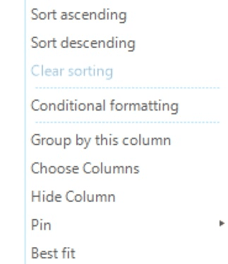
The Column context menu is the same for all column header cells in a table (Figure 28). It provides access to the following set of options:
- Sort ascending
-
Option to sort the selected column in ascending order.
- Sort descending
-
Option to sort the selected column in descending order.
- Clear sorting
-
Option to clear any sorting from the selected column.
- Conditional formatting
-
Option to open a window where the user can set the rules for formatting the content of the columns based on specific rules. See later on for more details.
- Group by this column
-
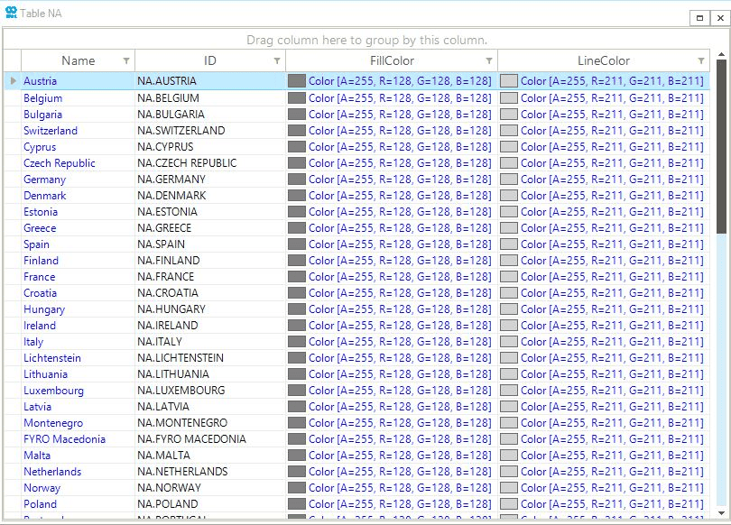
Option to group the entire table based on a selected column. The table can also be grouped by pressing the left mouse button and dragging the selected column above the table headers. The table can be ungrouped by dragging the grouped column back to the header row. Multiple cascading groups can be created.
- Choose columns
-
Option to open a window with all the possible column entries for the current table. The user can add the column entries by double-clicking on the column entry names.
- Hide column
-
Option to hide the selected column in the table.
- Pin
-
Option to unpin or pin to the left or right side of a table the selected column.
- Best fit
-
Option to adjust all columns width.
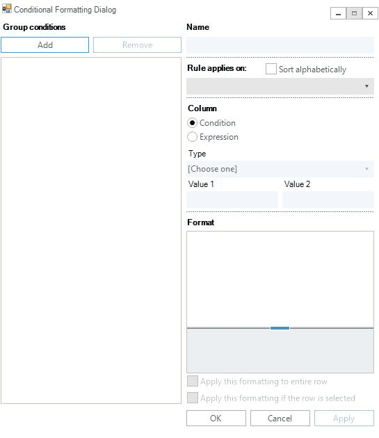
Conditional formatting allows the user to selectively format and style the content of rows and cells based on specific conditions and expressions (Figure 29). Multiple rules can be defined or removed from a table. Each rule must have a unique name, and must apply to a certain column. Rules must be developed based on predefined conditions (e.g., equal, greater, between value one and value two) or user defined expressions and involved up to two reference values. The user can format multiple aspects like the font used in cells and rows, the text alignment, the font color or the background color.
Finally, the Row context menu is accessed by right-clicking on any cell of a table (Figure 30). This context menu might slightly vary according to the cell selected.
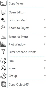
In general, Row context menu provides the following options, and have other object related entries:
- Copy Value
-
Option to copy the value of the selected cell.
- Open Editor
-
Option to open the property editor for changing properties associated to the object link to the row of the table.
- Select in Map
-
Option to select the object link to the cell in one of the opened map view windows.
- Zoom to Object
-
Option to select the map view window where to zoom to the object linked to the selected cell.
- Scenario event
-
Option to select from a list of possible events an option to add the object in the active simulation scenario.
- Plot Window
-
Option to select the chart to create based on a list associated to the type of object selected.
- Filter Scenario Events
-
Option to create a filter to create subsets of events.
- Sub
-
Option to open the property editor for the subsystem associated to the object and to create charts for such subsystem.
- Zone
-
Option to open the property editor for the subsystem associated to the object and to create charts for such subsystem.
- Group
-
Option to to create a new group by the selected object or add the object to an existing group.
The very last element available in the Table tab is the button PLG, which gives access to a table describing the polygons available in the active project with their properties. It allows the user to personalize each polygon for the name, visibility, color, and other geographic aspects (e.g., Figure 31).
3.4.2. Polygons
Polygons are cosmetic entities available only in Cartesian maps. As graphical objects in the map view, polygons help provide the user with background elements that support and enrich the understanding of the network.
The easiest way to incorporate polygons in a SAInt model is to import them from an external source. SAInt offers the possibility of importing polygons in shapefile format or from a Synergi project.
SAInt saves polygons in a dedicated file with extension *.plg along with possible attributes (stored in the Info property) and graphical properties like fill color, line color, and width, or line style.
By default, SAInt does not load polygons available in the project or network folders. The user must explicitly load polygons and save the project to restore them later. To load polygons from a *.plg file, select .
To remove polygons from the project, select the entry "Polygons" in the model explorer, and from the context menu, select "Unload Polygon(s)". This option does not delete the polygons but removes them from the active project.
Finally, polygons can be exchanged between projects. Either you share a copy of the *.plg file or from the context menu of the entry "Polygons" select the option "Export Polygon(s)" to save to a new polygon file.
SAInt has limited editing capabilities for polygons. But if the user needs to modify the geometry and the position of the vertices of a polygon, the coordinates and the list of vertices can be edited from the property editor after selecting the polygon and accessing the "Collection Editor" from the "Polygons" entry.
For more details on how to change the graphical properties of polygons, go to the How-To guide Edit Properties of Polygons.
3.5. View tab
The View tab of the ribbon bar collects a set of options to customize the dock panel of the GUI and to interact with certain windows. It is composed of two panels (Figure 32): the window panel and the layout panel.
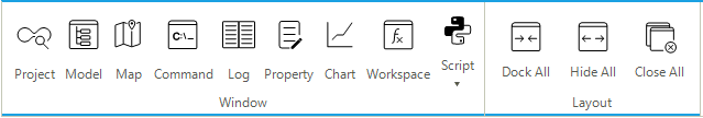
3.5.1. Window panel
The Window panel of the view tab allows the user to open previously closed windows of the GUI. A window is reopened in its default position. There are three exceptions to this default behavior: the map window, the script window, and the "Report Viewer" window. A map window is simply added to the available map windows in the dock panel. More than one map view (of the same type) can be available at the same time. The button Script allows to create a brand-new IronPython script or to open an existing script. The button Report Viewer allows to open a dedicated window where a simplified browser can render HTML pages created in SAInt as output of plugins or saved from the World-Wide Web.
The full list of options of the Window panel is available in Table 20.
| Icon | Options | Description |
|---|---|---|
|
Project |
Option to open the project explorer window. |
|
Model |
Option to open the model explorer window. |
|
Map |
Option to open a new map window. Multiple maps can be active in the dock panel at the same time. |
|
Node |
Option to open the node explorer window. |
|
Command |
Option to open the command window. |
|
Log |
Option to open the log window. |
|
Property |
Option to open the property editor window. |
|
Chart |
Option to open the chart window. |
|
Workspace |
Option to open the workspace window. |
|
Report Viewer |
Option to open the built-in HTML viewer to visualize and navigate local HTML pages. |
|
Script |
Option to open a brand-new or saved IronPython script editor window. |


3.5.2. Layout panel
The Layout panel of the View tab provides options to dock and open all windows in the dock panel, to close all floating windows in the dock panel, or hide all windows in the dock panel. The full list of options is available in Table 21.
| Icon | Options | Description |
|---|---|---|
|
Dock all |
Option to dock all the current windows. |
|
Hide all |
Option to hide all the current windows. |
|
Close all |
Option to close all the floating windows. |


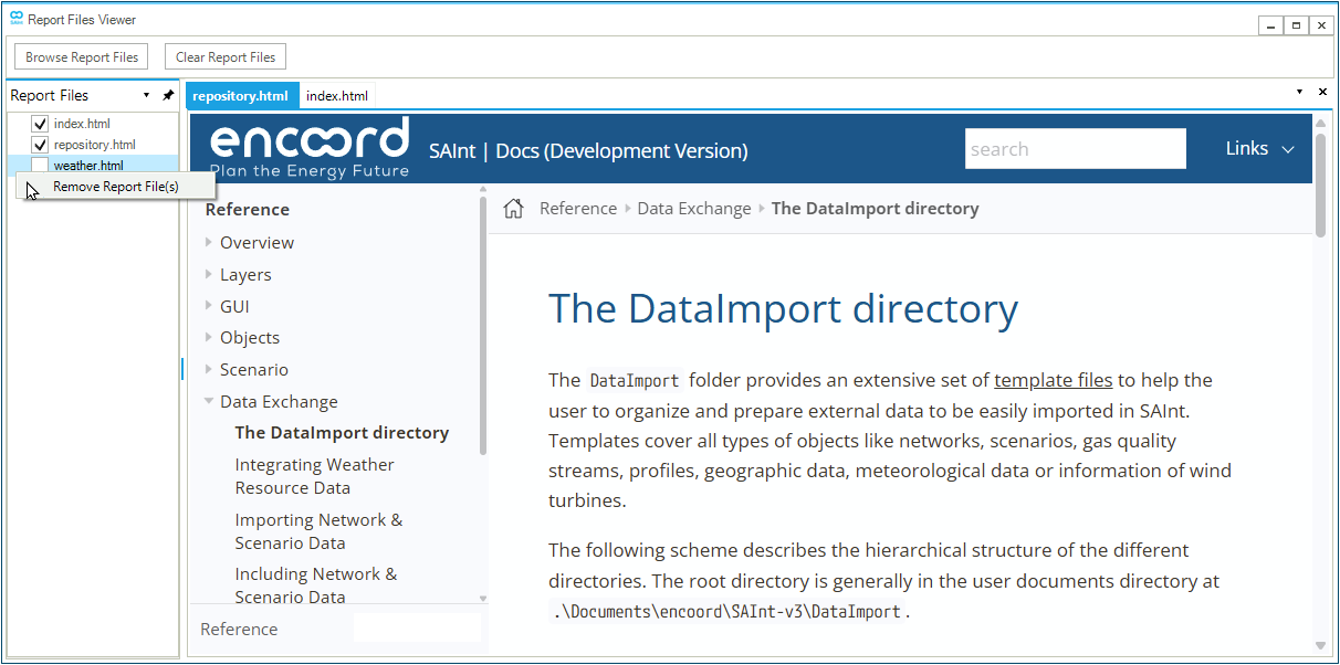
3.5.3. The Report Viewer
The "Report Viewer" is accessible from the tab "View" and the menu entry Report Viewer in the panel "Window". It provides the user with a SAInt built-in browser to visualize HTML documents created by running plugins, by exporting tables or pages downloaded from the World-Wide Web.
Figure 33 shows an example of the viewer after loading three pages called "index.html", "repository.html", and "weather.html". The user can load locally saved new pages using the button Browse Report Files, while the button Clear Report Files removes all loaded pages from the viewer. Available pages are listed in the window "Report Files". All ticked documents are loaded as single pages and displayed using different tabs on the right side of the viewer. An unticked document is a loaded page which is not displayed (e.g., page "weather.html" is loaded in the viewer but not visualized). The active page has its tab in blue, while loaded but not active pages have their tab in gray. The user can switch between loaded documents by clicking on the relevant tab. Pages can be removed from the viewer by using the context menu (i.e., by right-clicking) entry "Remove Report File(s)". And multiple pages can be selected by left-clicking the mouse while holding the "shift" or "CTRL" key on the keyboard. Finally, the black triangle icon and the "x" icon on the top-right of the area where a HTML page is visualized allow to select the active page from a drop-down list, and to close a page in the viewer (i.e., it is the equivalent of unticking the page from the list on the left).
3.6. Tools tab
The Tools tab of the ribbon bar provides access to capabilities for advanced functions and Python plugins.
Advanced tools are specific SAInt functionalities designed to carry out complex tasks and are directly available from the GUI and hardcoded into the SAInt dll. The first tool introduced with release 3.7 of SAInt is the "connectivity tool", which checks on the phase connectivity in an electric network so that the user is pointed to possible issues related to differences in the selected phases for branches or externals in 3-phase systems. This tool can identify situations like a line on a single-phase connected at both ends to 3-phase lines, or externals on a certain single-phase linked to a node attached to a 3-phase line. A lot of these phase discontinuities lead to numerically unsolvable problems, exceptions, or errors in the solver. To access the connectivity tool select (Figure 34). the level of logging for the tool can be set in the general settings of SAInt.
Plugins are external, self-contained executables developed in Python to process SAInt models or data. A plugin bundles all necessary Python packages, GUI elements, and executables to perform a specific analysis. The menu allows to launch any of the installed plugins and provides access to the general settings tab section Plugin Settings, from where plugins can be installed or removed. Plugins take advantage of SAInt-API functions and calls, along with functions provided by third-parties packages. Examples of plugins are available from the SAInt Community and SAInt Forum. The "contingency analysis" plugin, available from the SAInt Forum, showcases the use of this functionality. Given an electric system and a scenario, the plugin performs a contingency assessment where a set of objects (specified in the config file of the plugin) is removed from the system and the scenario is executed to check if the remaining part of the network fails or it is still able to cover the needs of the connected demands. For example, the plugin can be used to carry out a systematic study of an N-1 (or N-m with m equal to 1, or 2, or 3, etc.) contingency study.
SAInt allows executing multiple plugins simultaneously, as well as launching multiple instances of the same plugin. It is possible to use SAInt when long-running plugins are running. All encoord-authored plugins, available on the Forum, operate on copies of networks and scenarios, so multiple plugins trying to edit the same network or scenario is not a concern. User-authored plugins may lack this design feature, causing problems, triggering data changes, or making parallel execution of multiple plugins or instances of the same plugin impossible.
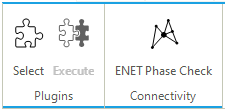
3.7. Help tab
The Help tab of the ribbon bar allows the user to access SAInt’s community, documentation material and the support team in encoord (Figure 35). The Help tab has five panels: documentation, community, support, license, and about.
The first time the user opens SAInt, the Help tab and the button "What’s New" are highlighted in the documentation panel. The user is invited to click on the "What’s New" button to access section three of the "Welcome" page summarizing the major changes to the new release of SAInt. At the end of the section, the user has also a shortcut to the full release notes. The highlight option is only available the first time SAInt is launched.
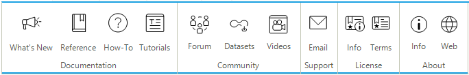
3.7.1. Documentation panel
The Documentation panel collects functions related to the local copy of SAInt documentation. The learn more menu option may not be yet available in this release. In general, the documentation is quickly accessible by pressing the keyboard key F1 in any SAInt window or over any SAInt graphical element. This action will redirect the user to the specific topic for that element inside the reference guide. The full list of options is available in Table 22.
| Icon | Options | Description |
|---|---|---|
|
What’s New |
Option to navigate to the "What’s New" section of the documentation. It contains information on all new features and functionalities included in the present release of SAInt. |
|
Reference |
Option to navigate to the Reference section of the documentation. It provides the user with an overview of SAInt and contains information on different components (e.g., GUI, API, scenarios etc.) of the present release of SAInt. |
|
How-to |
Option to navigate to the how-to guides section of the documentation. It provides the user with step-by-step instructions to complete a specific task (e.g., how to add an external to a node etc.) using SAInt. The how-to guides are divided into generic, electric, gas, and combined sections and are updated every new release of SAInt. |
|
Tutorial |
Option to navigate to the tutorial section of the documentation. It contains set of tutorials related to address a problem (e.g., create a gas network, create a DCUCOPF scenario, executing a DynamicGas simulation etc.) in SAInt. The tutorials are updated with the new releases of SAInt. |
|
Learn More |
Option to navigate to the learn more section of the documentation. It contains detailed, advanced technical information on SAInt mathematical formulation of the models of the different objects. |


3.7.2. Community
The community panel allows access to the online forum, where the users meet to discuss SAInt and of how to use SAInt to solve their challenges. The community can also take advantage of open-source model-ready datasets to speed up research and problem-solving in integrated planning and energy system modelling. Some video guides are also accessible to complement SAInt’s documentation. Table 23 summarizes the available functionalities.
| Icon | Options | Description |
|---|---|---|
|
Forum |
Option to open the online community forum to meet other SAInt users. |
|
Dataset |
Option to access the forum page where download model ready datasets for SAInt. |
|
Videos |
Option to navigate to online video resources on th euse of SAInt. |


3.7.3. Support panel
The Support panel allows the user to contact the encoord’s support team. The full list of options is available in Table 24.
| Icon | Options | Description |
|---|---|---|
|
Option to open a pre-filled email that will be send to encoord’s support team. |

|
Another option to provide feedback to encoord is by sending an exception email. A window will pop up if SAInt detects an error, in which the user can describe the details of the issue. This email contains the exception details and the SAInt version. The encoord support team will collect the error details and contact the user with a solution. |
3.7.4. License panel
The license panel of the Help tab allows to check and read all necessary information and terms of the license of SAInt. Through this panel is also possible to request the renewal of an existing license. The full list of options is available in Table 25.
| Icon | Options | Description |
|---|---|---|
|
Info |
Option to open the |
|
Terms |
Option to open a document containing the software license agreement. |


3.7.5. About panel
The about panel of the help tab shows the version of SAInt in use, and provides the link to encoord website. The full list of options is available in Table 26.
| Icon | Options | Description |
|---|---|---|
|
Info |
Option to open a splash screen showing the installed SAInt version. The splash screen can be closed by clicking on it. |
|
Web |
Option to open the encoord website in the default browser. |


3.7.6. Exception window
SAInt offers the user the option to share technical data directly with the "Customer Support Service" of encoord by means of the "Exception!" window, a pop-up window triggered whenever an action is throwing an error in the expected behavior of SAInt-GUI. The "Exception!" window asks the user to provide a valid e-mail and optionally to specify the name and a short description of the event leading to the exception (Figure 36). The technical details of the exception are available for inspection and are shared with the "Customer Support Service".
If available, the name of the network, the name of the scenario or the name of the profiles file are recorded as well in the exception message, and shared with Customer Support. This helps in debugging and facilitate communication with the user. No data, network’s or scenario’s details are transferred.
An error triggered by a Python script using the API or by an IronPython script in the GUI is handled by SAInt respectively by logging the Python exception messages to an external log file or by using a pop-up window with information of the IronPython script problem.