Electric Scenarios

An electric scenario describes the operation of an electric network according to conditions specified in the scenario properties and events. An electric scenario can determine network operational parameters such as power flow quantities, nodal voltages, generation dispatch, and shadow prices across the network, to name a few. The conditions at which these variables are evaluated are specified by the events of the electric scenario, or adopted by default values specified at the network level. The properties and settings of an electric scenario define aspects such as the time span, resolution, and numerical tolerances adopted for the solution while the mathematical equations being respected are relevant to the type of scenario applied.

There are two broad categories of electric scenarios: steady state, and quasi-dynamic, where the distinguishing factor is a steady state looks at a single timestep, and the latter multiple timesteps. Additional distinctions, such as optimality, the linear approximation notated as DC, or the unit commitment application, further characterize these two broad categories. The direct current unit commitment optimal power flow scenario (DCUCOPF) and the capacity expansion model scenario (CEM) are treated independently in this documentation, due to the additional optimization criteria that characterizes these scenarios.

Scenario’s properties can be defined either in the "Scenario Dialog" when creating a new scenario or through the "Property Editor", once the scenario is created.

1. Steady scenarios

The steady scenario represents the system at a single time instance in a power flow equilibrium condition. It can be used to analyze the operation of an electric network at a particular dispatch, to assess the voltage magnitudes and angles. Table 1 provides an overview of the five different types of steady scenarios available in SAInt.

Table 1. Steady electric scenario types.
Scenario type	Description
`SteadyACPF`	Balanced Single Time Step AC-Power Flow Simulation. Single time step, phase-balanced, steady-state, alternating current (AC) power flow simulation. Simulation of power flows in an electric network considering: voltage drop/change equations across the from- and to-node of lines and transformers; nodal AC balance equations; reactive power limits of generators; a distributed active power compensation for multi-generator network models. The resulting mathematical model is a set of non-linear equations solved using a Newton-Raphson linearization algorithm.
`SteadyACOPF`	Balanced Single Time Step AC-Power Flow Optimization. Single time step, phase-balanced, steady-state alternating current (AC) power flow optimization. Optimization of active power generation dispatch costs (objective function) in an electric network subject to: voltage drop/change equations across the from- and to-node of lines and transformers; nodal AC balance equations; nodal voltage limits; active and reactive power limits of generators; current, active power, and apparent power limits of lines and transformers. The resulting mathematical model is a non-linear optimization model (NLP) solved with Gurobi’s LP-Solver using a sequential linear programming algorithm (SLP).
`SteadyUACPF`	Unbalanced Single Time Step AC-Power Flow Simulation. Single time step, single-, two- or three-phase unbalanced, steady-state, alternating current (AC) power flow simulation. Simulation of power flows in an electric network considering: voltage drop/change equations per phase for lines and transformers; nodal AC balance equations per phase; generator reactive power limits; a distributed active power compensation model for multi-generator networks; single-, or two-phase-, wye-, or delta-connected loads. The resulting mathematical model is a set of non-linear equations which is solved using a Newton-Raphson linearization algorithm.

Any (quasi-)dynamic scenario can not last longer than 68 years. SAInt will inform the user of this violation and prevent the scenario from being created.

1.1. Scenario settings

The properties of a steady scenario allow the user to specify solver settings, time-related information, general attributes, and chart visualization options when accessed using the property editor. Solver settings provide control over the residual tolerances and the maximum number of iterations admitted during the numerical solution of the electric power flow problem. The time settings associated with a steady scenario are simply the time of the single instance, although the properties as related to quasi-dynamic scenarios will still be visible to the user. Table 2 provides an overview of the solver properties for a steady scenario, while Table 3 shows the time-related properties.

In case of big power systems, the computation load and the speed of convergence for a solution may be quite challenging factors to address. SAInt implements a light loading start methodology in ACPF simulations to facilitate the solver in finding a solution. The relevant parameters are described in Table 4. Consider the How-To "Light Loading Start in ACPF simulations" for a description of the steps to activate and fine-tune the options.

SAInt uses Gurobi (https://www.gurobi.com/) as solver for optimization problems related to ACOPF scenarios. The user can specify a set of Gurobi settings either in the SAInt-GUI or using the API when defining a scenario. For more details check Table 2 and the Gurobi’s Parameter Reference online page.

Table 2. Solver settings of a steady scenario.
Display Name	Description
`ResidualTolerance`	Residual tolerance applied to conclude on success of the solution method.
`MaxResidualIterations`	Maximum number of iteration steps for linearization. The default is 50, and the minimum is 5.
`MaxControIterations`	The maximum number of iteration steps for constraint and control handling. The default is 10 steps. It could be zero.
`MaxTransformerTapIterations`	The maximum number of iteration steps for changing the tap position of a transformer. The default is 10 steps. It could be zero.
`LinearSolverEngine`	Select the type of linear solver to use. Choices are: "Pardiso", "SparseLU", and "KLU". Default is "SparseLU".
`SolverTimeLimit`	Set the time limit for the solver in seconds. Default value is 3600 seconds (i.e., one hour).
`SoftMemLimit`	Gurobi setting: set the memory limit in GB used by the optimization solver. The default value is infinite like in Gurobi. Accepted values are double numeric values between 0 and positive infinity.
`PreSolve`	Gurobi setting: set the presolve level for the optimization solver. The default value is -1 like in Gurobi. Accepted values are integer numeric values in {-1; 0; 1; 2}.
`AggFill`	Gurobi setting: set the allowed fill during presolve aggregation for the optimization solver. The default value is -1 like in Gurobi. Accepted values are integer numeric values in [-1; 2,000,000,000].
`NumericFocus`	Gurobi setting: set the numeric focus of the optimization solver. The default value is 1, while Gurobi uses a default of 0 (i.e., automatic choice). SAInt value of one increases the focus towards being more careful in numerical calculations. Accepted values are integer numeric values in {0; 1; 2; 3}.
`Seed`	Gurobi setting: set a random seed for the optimization solver. The default value is 0 like in Gurobi. Accepted values are integer numeric values in [-1; 2,000,000,000].
`Threads`	Gurobi setting: set the number of CPU threads used by the optimization solver. The default value is 0 and Gurobi sets automatically the value. Accepted values are integer numeric values defined by the maximum number of threads provided by the CPU of the computer used.
`OutputFlag`	Gurobi setting: set if to suppress Gurobi logging, including the license connection parameters like in Gurobi with the settings "OutputFlag" or "LogToConsole". Accepted values are integer numeric values in {0; 1}. Default is 1, which indicates to log the Gurobi output.

Table 3. Time settings of a steady scenario.
Display name	Description
`StartTime`	This is the time of the single instance that is executed with the steady scenario.
`EndTime`	This property is not relevant to the steady scenario, but it will always be visible and show a value one hour later than the `StartTime`.
`TimeWindow`	The steady scenario has no length of time because it represents a single instance in time. However, this value will still show the difference between `EndTime` and `StartTime`, which will be a fixed one-hour duration due to the automatic setting of the `EndTime` property.
`TimeStep`	The `TimeStep` property is not relevant to the steady scenario, but it will be visible and show the default value of 60 minutes.
`StepsTimeWindow`	The `StepsTimeWindow` property is not relevant to the steady scenario, but it will be visible and show a default value of 1.
`IniState`	Name of the scenario whose terminal state is used as the initial state for the current scenario. Default is set to none. This is an optional property, and not relevant for a steady scenario.

Table 4. Light loading start options for a steady state ACPF scenario.
Display name	Description
`LightLoadingLoadFactor`	Light loading load reduction factor for the first load reduction step. All demand and shunt active and reactive power loadings will be multiplied by this factor. The validity range is [0;1]. Default value is 0.3.
`LightLoadingLoadSteps`	Number of light loading load reduction steps until full loading. If set to 0, no load reduction is performed. If greater than 1, then the load factor will increase with an increment of (1-`LightLoadingLoadFactor`)/`LightLoadingLoadSteps`. Default value is 0 (i.e., no light loading reduction). The validity range is [1;20].
`LightLoadingResidualTolerance`	Residual tolerance during light loading reduction steps. Default value is 1, and the validity range is [10^-5;10⁴].

2. Quasi-dynamic scenarios

Quasi-dynamic electric scenarios (AC and DC) comprise power flow (PF) and optimal power flow (OPF) simulations. A succession of steady scenarios comprises a quasi-dynamic scenario. Quasi-dynamic AC/DC PF scenarios are a succession of independent steady simulations, while quasi-dynamic AC/DC OPF scenarios are a succession of optimizations where generator constraints are considered between consecutive timesteps. Table 5 provides an overview of the four different types of quasi-dynamic scenarios available in SAInt.

When solving a quasi-dynamic scenario, one or more of the independent steady state steps may fail. SAInt informs the user of the failure with a specific pop-up window, and by turning red, the status of the "solver indicator" in the status bar is updated. Furthermore, SAInt registers which time steps did not converge and details such time steps in the log file of the simulation.

Table 5. Quasi dynamic electric scenario types.
Scenario type	Description
`QuasiDynamicACPF`	Balanced Multi Time Step AC-Power Flow Simulation. Multi time step, phase-balanced, steady-state, alternating current (AC) power flow simulation. Simulation of power flows in an electric network considering: voltage drop/change equations across the from- and to-node of lines and transformers; nodal AC balance equations; reactive power limits of generators; a distributed active power compensation for multi-generator network models. The resulting mathematical model is a set of non-linear equations solved using a Newton-Raphson linearization algorithm.
`QuasiDynamicACOPF`	Balanced Multi Time Step AC-Power Flow Optimization. Multi time step, phase-balanced, steady-state alternating current (AC) power flow optimization. Optimization of active power generation dispatch costs (objective function) in an electric network subject to: voltage drop/change equations across the from- and to-node of lines and transformers; nodal AC balance equations; nodal voltage limits; active and reactive power limits of generators; current, active power, and apparent power limits of lines and transformers. The resulting mathematical model is a non-linear optimization model (NLP) solved with Gurobi’s LP-Solver using a sequential linear programming algorithm (SLP).
`QuasiDynamicUACPF`	Unbalanced Multi Time Step AC-Power Flow Simulation. Multi time step, single-, two- or three-phase unbalanced, steady-state, alternating current (AC) power flow simulation. Simulation of power flows in an electric network considering: voltage drop/change equations per phase for lines and transformers; nodal AC balance equations per phase; generator reactive power limits; a distributed active power compensation model for multi-generator networks; single-, or two-phase-, wye-, or delta-connected loads. The resulting mathematical model is a set of non-linear equations which is solved using a Newton-Raphson linearization algorithm.

2.1. Scenario settings

The properties of a quasi-dynamic scenario allow the user to specify solver settings, time-related information, general attributes, and chart visualization options when accessed using the property editor. Solver settings provide control over the residual tolerances and the maximum number of iterations admitted during the numerical solution of the quasi-dynamic electric problem formulation. Voltage formulation settings can be optionally selected. The time settings for a quasi-dynamic scenario define the optimization time window, the start time and the end time, the time step, and an optional scenario providing the initial conditions, constituting the operational snapshot of the system prior to the beginning of the scenario. Table 6 provides an overview of the solver’s properties for a quasi-dynamic scenario, while Table 7 shows the time-related properties.

In case of big power systems, the computation load and the speed of convergence for a solution may be quite challenging factors to address. SAInt implements a light loading start methodology in ACPF simulations to facilitate the solver in finding a solution. The relevant parameters are described in Table 8. Consider the How-To "Light Loading Start in ACPF simulations" for a description of the steps to activate and fine-tune the options.

SAInt uses Gurobi (https://www.gurobi.com/) as solver for optimization problems related to ACOPF scenarios. The user can specify a set of Gurobi settings either in the SAInt-GUI or using the API when defining a scenario. For more details check Table 6 and the Gurobi’s Parameter Reference online page.

Table 6. Solver settings of a quasi-dynamic electric scenario.
Display name	Description
`ResidualTolerance`	The residual tolerance for linearization steps.
`MaxResidualIterations`	Maximum number of iteration steps for linearization. The default is 50, and the minimum is 5.
`MaxControIterations`	The maximum number of iteration steps for constraint and control handling. The default is 10 steps. It could be zero.
`MaxTransformerTapIterations`	The maximum number of iteration steps for changing the tap position of a transformer. The default is 10 steps. It could be zero.
`LinearSolverEngine`	Select the type of linear solver to use. Choices are: "Pardiso", "SparseLU", and "KLU". Default is "SparseLU".
`SolverTimeLimit`	Set the time limit for the solver in seconds. Default value is 3600 seconds (i.e., one hour).
`SoftMemLimit`	Gurobi setting: set the memory limit in GB used by the optimization solver. The default value is infinite like in Gurobi. Accepted values are double numeric values between 0 and positive infinity.
`PreSolve`	Gurobi setting: set the presolve level for the optimization solver. The default value is -1 like in Gurobi. Accepted values are integer numeric values in {-1; 0; 1; 2}.
`AggFill`	Gurobi setting: set the allowed fill during presolve aggregation for the optimization solver. The default value is -1 like in Gurobi. Accepted values are integer numeric values in [-1; 2,000,000,000].
`NumericFocus`	Gurobi setting: set the numeric focus of the optimization solver. The default value is 1, while Gurobi uses a default of 0 (i.e., automatic choice). SAInt value of one increases the focus towards being more careful in numerical calculations. Accepted values are integer numeric values in {0; 1; 2; 3}.
`Seed`	Gurobi setting: set a random seed for the optimization solver. The default value is 0 like in Gurobi. Accepted values are integer numeric values in [-1; 2,000,000,000].
`Threads`	Gurobi setting: set the number of CPU threads used by the optimization solver. The default value is 0 and Gurobi sets automatically the value. Accepted values are integer numeric values defined by the maximum number of threads provided by the CPU of the computer used.
`OutputFlag`	Gurobi setting: set if to suppress Gurobi logging, including the license connection parameters like in Gurobi with the settings "OutputFlag" or "LogToConsole". Accepted values are integer numeric values in {0; 1}. Default is 1, which indicates to log the Gurobi output.

Table 7. Time settings of a quasi-dynamic electric scenario.
Display name	Description
`StartTime`	The start time of the scenario. This is the first time step in a scenario. The default is to set the calendar day and hour of when the scenario is created by the user.
`EndTime`	The end time of the scenario. This is the final time step in a scenario. The default is to set the hour and a plus one calendar day of when the scenario is created.
`TimeWindow`	The total simulation time window or the total amount of time in a scenario (i.e., the difference between `EndTime` and `StartTime`).
`TimeStep`	A time step is a fraction of the scenario time window used for discretizing the scenario time window into distinct time points which are calculated for the variables. The time window is a multiple of the time step, i.e. `TimeWindow` divided by `TimeStep` must be an integer greater than or equal to one. The default is to have 15 minutes timestep.
`StepsTimeWindow`	The number of time steps for the scenario time window (i.e. `TimeWindow` divided by `TimeStep`).
`IniState`	Name of the scenario whose terminal state is used as the initial state for the current scenario. This is an optional property, and the default is set to none. The property is in the "General" section of the property editor.

Table 8. Light loading start options for a quasi-dynamic ACPF scenario.
Display name	Description
`LightLoadingLoadFactor`	Light loading load reduction factor for the first load reduction step. All demand and shunt active and reactive power loadings will be multiplied by this factor. The validity range is [0;1]. Default value is 0.3.
`LightLoadingLoadSteps`	Number of light loading load reduction steps until full loading. If set to 0, no load reduction is performed. If greater than 1, then the load factor will increase with an increment of (1-`LightLoadingLoadFactor`)/`LightLoadingLoadSteps`. Default value is 0 (i.e., no light loading reduction). The validity range is [1;20].
`LightLoadingResidualTolerance`	Residual tolerance during light loading reduction steps. Default value is 1, and the validity range is [10^-5;10⁴].

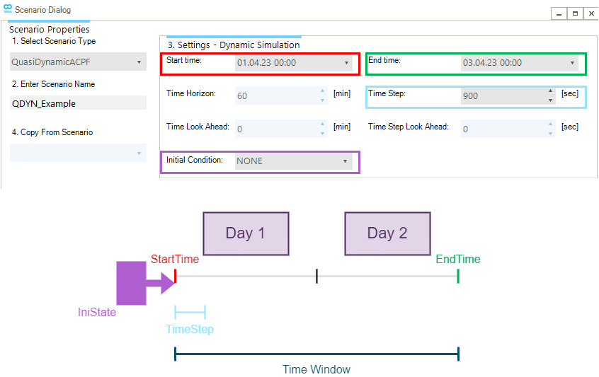
Figure 1 shows an example of the time settings and the associated graphical description of a quasi-dynamic ACPF scenario as available in the Scenario Dialog window.

Figure 1. Example of time settings and graphical description of a quasi-dynamicACPF scenario.

3. Best Practices for convergence in AC Power Flow scenarios

Solving an AC Power Flow (ACPF) scenario becomes increasingly challenging as the size and complexity of the network model increase. Large and complex networks contain many state variables and non-linear governing equations, making numerical convergence highly sensitive to modeling choices and initial conditions.

To support users in obtaining a converged solution across a wide range of network sizes and complexities, SAInt provides several solver initialization and modeling options. This document explains the underlying principles and provides guidance on selecting the appropriate options to improve convergence behavior based on general network characteristics and solver behavior.

3.1. Background: why convergence can be challenging

An ACPF simulation solves a system of non-linear algebraic equations that describes the steady-state electrical behavior of the network. These equations are typically solved using iterative numerical methods, which repeatedly linearize the equations around a current estimate of the solution.

The choice of initial values for the solution variables—primarily voltage magnitudes and voltage phase angles—has a significant influence on:

whether the model converges at all;
how many iterations are required;
whether the solution oscillates or diverges.

As network size and complexity increase:

the number of variables and equations grows;
the system becomes more strongly non-linear;
poor initial guesses are more likely to lead to divergence.

Therefore, selecting a good starting point and appropriate convergence-supporting modeling options becomes increasingly important for large or heavily loaded systems.

3.2. Solver Initialization Options

3.2.1. Flat Start

With a "Flat Start", all bus voltage magnitudes are initialized to 1.0 p.u., and all voltage phase angles are set to 0 degrees.

Characteristics

Simple and robust for small or lightly loaded networks.
Requires no prior solution.
Useful during early model development or for simple test cases.

Limitations

May require many iterations.
Often fails to converge for large, heavily loaded, or stressed networks.

Recommendation

Use Flat Start primarily for small networks or when no previous solution is available.

3.2.2. Warm Start

A "Warm Start" uses the converged steady-state solution of an ACPF simulation as the initial guess for another ACPF simulation of the same network model.

In SAInt, this is achieved by selecting the solution of a previous steady-state scenario as the initial state of the current scenario. The solver loads the corresponding results from the associated econ file and uses them as the starting point for the active scenario.

Characteristics

Provides verified initial voltage magnitudes and phase angles.
Can significantly improve convergence speed and robustness.
Particularly effective when the scenario settings and network configuration do not differ substantially from the previous steady-state scenario.

Additional Notes

Warm Start capability is automatically used between consecutive time steps of a quasi-dynamic ACPF scenario.
Performance gains are greatest when changes between scenarios are small (e.g., gradual load changes or minor topology variations).

Recommendation

Use Warm Start whenever a suitable converged solution is available. This is the preferred initialization method for scenario analysis, contingency studies, and time-series simulations.

3.2.3. Load Conditioning

"Light Loading" is a continuation-based approach that can improve convergence behavior by gradually increasing system loading.

In this method, the active and reactive power of demands and shunt elements are initially reduced. The solver first computes a solution for this lightly loaded system using a Flat Start. The resulting solution is then used as an initial guess for a slightly higher loading level. This process is repeated until the full system loading is reached.

Key Features

Reduces system stress during early iterations.
Helps guide the solver toward a feasible solution path.
The user can configure the number of light loading steps before solving the fully loaded system.

Typical Use Cases

Very large networks.
Heavily loaded or stressed operating conditions.
Models that fail to converge with Flat Start or Warm Start alone.

Recommendation

Use Light Loading as a powerful convergence aid for difficult scenarios. It is especially effective when combined with advanced voltage control modes (covered below).

3.2.4. Voltage Control Modeling

The VoltageControlMode setting determines:

how the voltage magnitude setpoint of voltage-controlling devices (e.g. generators, prosumers, storage units) is mathematically represented, and
how reactive power limit violations are handled during the iterative solution process.

This choice has a strong impact on convergence behavior, especially in networks with many voltage-controlling elements. Note, this does not materially impact the physical voltage control mode of a generator, only the representation during the solve process.

VoltageControlMode can take the following three states: "Normal", "SlopedSoftLimit" and "SlopedHardLimit".

Normal

In "Normal" mode, voltage control is described by the equation: V_m = V_m,set
where:

V_m is the voltage magnitude variable;
V_m,set is the voltage magnitude set point.

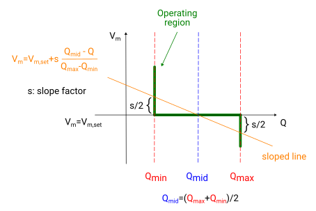
This corresponds to a horizontal line in the V_m-Q diagram (Figure 2).

Figure 2. V_m-Q diagram describing the operating points of a generator in terms of voltage magnitude (V_m) and reactive power (Q). The green line shows the generator’s feasible operating region within its reactive power limits, while the orange line approximates the operating region with a sloped line.

Reactive power limit switches (i.e., transitions between voltage control and Q_min/Q_max control) are only performed once the residual of the previous iteration is below 1, meaning the solution estimate is already close to convergence.

Characteristics:

Enforces the voltage setpoint strictly.
Can lead to very large reactive power injections in early iterations.

Limitations:

Large initial reactive power flows may cause divergence.

Recommendation

Use Normal mode for well-conditioned networks or after a stable solution has already been obtained using more robust modes.

SlopedSoftLimit

improves convergence by relaxing voltage control during early iterations. Voltage control is described by (see Figure 2): V_m = V_m,set + s (Q_mid - Q) / (Q_max - Q_min)
where:

Q_mid is equal to the average of Q_max and Q_min (i.e., (Q_max+Q_min)/2);
Q is the reactive power variable;
Q_max and Q_min are the maximum and minimum reactive power, respectively;
s is the slope factor.

Key Characteristics

The slope factor starts with a value equal to the scenario property StartSlopeFactor (default value is 0.05) in the first iteration and is gradually reduced toward the scenario property MinSlopeFactor (default value is 0) when the residual of the previous iteration is below 1.
Excessive reactive power flows during initial iterations are limited.
The reactive power range [Q_min,Q_max] of generators is temporarily enlarged internally, proportional to the slope factor.
Voltage control switches for reactive power limit violations of the enlarged reactive power range are only performed once the residual of the previous iteration is below 1.
The user can set the minimum enlargement of the reactive power range by specifying a value for the scenario property MinSlopedSoftLimit (default value is 0). The solver starts from an enlargement of the reactive power range of 100% for all voltage controlling externals and gradually reduces this enlargement to MinSlopedSloftLimit. Please note that MinSlopedSoftLimit only has an effect if the scenario property MaxControlIterations is greater than 0.

Recommendation

Use SlopedSoftLimit as the default choice for large or difficult networks. It provides a good balance between robustness and accuracy.

SlopedHardLimit

is similar to SlopedSoftLimit, but with stricter enforcement of reactive power limits.

Differences Compared to SlopedSoftLimit:

Reactive power limits are not enlarged.

Recommendation

Use SlopedHardLimit when strict adherence to reactive power limits is required, while still improving convergence robustness compared to Normal mode.

3.2.5. Active Power Balancing

The way generators participate in balancing active power mismatches can significantly influence convergence. If only a small subset of generators participates in active power balancing, very large active power flows may occur in the areas where these generators are connected during early iterations. This can lead to numerical instability and divergence.

SAInt already provides the users with the ability to set participation factors with the PFSET property. However, this property fixes the participation of all generations in the final solution. To allow a broader participation of all generations during the solution process only, SAInt provides the SwitchParticipation option.

Behavior:

Initially, all generators participate in active power balancing.
This continues until the solver residuals fall below the specified residual tolerance.
Once the solution is sufficiently close to convergence, participation is switched back to only those generators intended to participate according to the model definition.

Recommendation

Enable SwitchParticipation for large and heavily loaded networks where only a few generators are intended to participate in balancing the active power mismatch.

3.3. Summary of Recommended Strategy

Prefer "Warm Start" over "Flat Start" whenever possible.
Use "Light Loading" for large, stressed, or difficult-to-converge networks.
Select SlopedSoftLimit or SlopedHardLimit voltage control modes for improved robustness.
Enable SwitchParticipation to stabilize early iterations in large systems.
Once a stable solution is obtained, stricter control modes can be re-enabled if needed.

4. DCUCOPF scenarios

The DCUCOPF is a scenario for optimizing the decisions on unit commitment and economic dispatch considering generator, storage, and transmission constraints using a linear approximation of the non-linear AC power flow equations ( i.e., (a) nodal voltage = nominal voltage, (b) resistance << reactance, (c) negligible voltage phase angle difference across lines and transformers). Each optimization time horizon can have a look-ahead period to inform decisions that influence the network’s state beyond the end of the optimization window.

The resulting mathematical model is a linear, mixed-integer optimization model (MIP) solved with Gurobi’s MIP-Solver using a rolling time horizon with look-ahead method.

4.1. Scenario settings

The properties of a DCUCOPF scenario allow the user to specify solver and time-related information, as well as general attributes and chart visualization options. Solver settings provide control over the solver type, the solver model, the time limit, and the relative MIP gap. Optionally, the user can write to an external file the linear programming problem for the optimization of the active model. The time settings for a DCUCOPF scenario define, as for a quasi-dynamic scenario, the optimization time window, the start time and the end time, the time step for the time horizon, and an optional scenario providing the initial conditions, constituting the operational snapshot of the system prior to the beginning of the scenario. Furthermore, the user can specify the time look ahead, the time step look ahead, and the time horizon. Table 9 provides an overview of the solver’s properties for a quasi-dynamic scenario, while Table 10 shows the time-related properties.

SAInt uses Gurobi (https://www.gurobi.com/) as solver for optimization problems. The user can specify a set of Gurobi settings either in the SAInt-GUI or using the API when defining a scenario. For more details check Table 9 and the Gurobi’s Parameter Reference online page.

For DCUCOPF scenarios, the user is asked to confirm any new execution that overwrites an existing solution. This extra check is meant to prevent launching a long optimization run or accidentally overwriting a solution.

Table 9. Solver settings of a DCUCOPF scenario.
Display name	Description
`OptimizationSolverEngine`	Solver type to use for solving the LP and MIP. The only available option is Gurobi. Other options may be available in future releases.
`OptimizationProblemType`	The type of solver model to use. Choices are: MIP, LP and QP. Default is MIP.
`LinearSolverEngine`	Select the type of linear solver to use. Choices are: "Pardiso", "SparseLU", and "KLU". Default is "SparseLU".
`SolverTimeLimit`	The time limit for the DCUCOPF solver. If the relative MIP gap is not achieved within the solver time limit, the latest solution found is considered as the result of the time horizon. Default is 3600 seconds.
`RelativeMipGap`	The relative MIP gap for branch and bound algorithm (i.e., relative difference between best integer objective and the best objective in the remaining unbranched nodes in the branch and bound tree). Default is 1.0E-3.
`WriteLPFile`	Indicates if an LP file of the optimization model should be generated. This file lists the objective functions and all the linearized equations. Default is to not generate the file.
`SoftMemLimit`	Gurobi setting: set the memory limit in GB used by the optimization solver. The default value is infinite like in Gurobi. Accepted values are double numeric values between 0 and positive infinity.
`PreSolve`	Gurobi setting: set the presolve level for the optimization solver. The default value is -1 like in Gurobi. Accepted values are integer numeric values in {-1; 0; 1; 2}.
`AggFill`	Gurobi setting: set the allowed fill during presolve aggregation for the optimization solver. The default value is -1 like in Gurobi. Accepted values are integer numeric values in [-1; 2,000,000,000].
`IntegralityFocus`	Gurobi setting: set the integrality focus of the MIP optimization solver. The default value is 1, while Gurobi uses a default of 0. SAInt requires Gurobi that the solver tries harder to avoid solutions that exploit integrality tolerances. Accepted values are integer numeric values in {0; 1}.
`NumericFocus`	Gurobi setting: set the numeric focus of the optimization solver. The default value is 1, while Gurobi uses a default of 0 (i.e., automatic choice). SAInt value of one increases the focus towards being more careful in numerical calculations. Accepted values are integer numeric values in {0; 1; 2; 3}.
`MIPFocus`	Gurobi setting: set the MIP focus of the optimization solver. The default is 0 like in Gurobi. Accepted values are integer numeric values in {0; 1; 2; 3}.
`Seed`	Gurobi setting: set a random seed for the optimization solver. The default value is 0 like in Gurobi. Accepted values are integer numeric values in [-1; 2,000,000,000].
`Threads`	Gurobi setting: set the number of CPU threads used by the optimization solver. The default value is 0 and Gurobi sets automatically the value. Accepted values are integer numeric values defined by the maximum number of threads provided by the CPU of the computer used.
`ImproveStartGap`	Gurobi setting: set the MIP gap at which to change the solution strategy of the optimization solver. The default value is 0 like in Gurobi. Accepted values are double numeric values between 0 and plus infinite.
`Heuristics`	Gurobi setting: set the fraction of time spent in feasibility heuristics by the optimization solver. The default value is 0.05 (i.e., the 5 % of the time) like in Gurobi. Accepted values are double numeric values in [0; 1].
`OutputFlag`	Gurobi setting: set if to suppress Gurobi logging, including the license connection parameters like in Gurobi with the settings "OutputFlag" or "LogToConsole". Accepted values are integer numeric values in {0; 1}. Default is 1, which indicates to log the Gurobi output.

Table 10. Time settings of a DCUCOPF scenario.
Display name	Description
`StartTime`	Start time of the scenario. It is the first time step in a scenario. The default is to set the calendar day and hour of when the scenario is created.
`EndTime`	End time of the scenario. It is the final time step in a scenario. The default is to set the hour and a plus one calendar day of when the scenario is created.
`TimeWindow`	The total amount of time in a scenario (i.e. the difference between `EndTime` and `StartTime`). This is a derived option. The time window cannot be bigger than 68 years.
`TimeHorizon`	The time horizon is a fraction of the scenario time window considered for a consecutive optimization in a DCUCOPF scenario. The time window is a multiple of the time horizon, i.e. `TimeWindow` divided by `TimeHorizon` must be an integer greater than or equal to one. This integer represents the number of consecutive optimizations for a DCUCOPF scenario. Each consecutive optimization covers a time interval of the scenario time window equal to the time horizon. Default is set to 60 minutes.
`TimeStep`	A time step is a fraction of the scenario time window used for discretizing the scenario time window into distinct time points which are calculated for the variables. The time window is a multiple of the time step, i.e., `TimeWindow` divided by `TimeStep` must be an integer greater than or equal to one. Default is set to 15 minutes. In DCUCOPF, SAInt uses the label "Time Step Horizon" to better clarify the concept.
`TimeLookAhead`	A look ahead, look ahead time, or time look ahead is a time duration added to the time interval considered in the consecutive optimization for a DCUCOPF scenario. It assists the mathematical model in finding a more realistic solution for the commitments of generators and the operation of storages close to the end of a time horizon as it indicates that the operation of the generators does not end at the end of the time horizon. The total time interval for a consecutive optimization is composed of the `TimeHorizon` and the `TimeLookAhead`. Default is set to zero minutes.
`TimeStepLookAhead`	The time step for the look ahead. It typically has a smaller time resolution or a longer time step than the time horizon. Default is set to zero minutes.
`IniState`	Name of the scenario whose terminal state is used as the initial state for the current scenario. Default is set to none. This is an optional property.
`ConsecutiveRuns`	Number of consecutive runs for a given time horizon and scenario time window (i.e., `TimeWindow` divided by `TimeHorizon`). This is a derived option.
`StepsTimeWindow`	The number of timesteps for the scenario time window (i.e., `TimeWindow` divided by `TimeStep`). This is a derived option.
`StepsTimeHorizon`	The number of time steps per time horizon (i.e., `TimeHorizon` divided by `TimeStep`). This is a derived option.
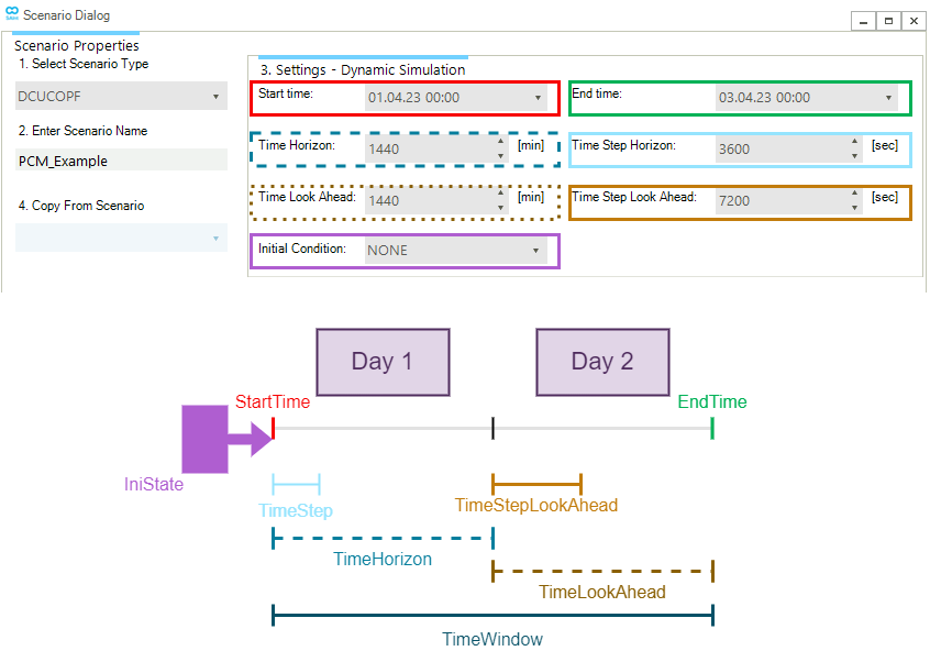
`StepsLookAhead`	The number of time steps per look ahead (i.e., `TimeLookAhead` divided by `StepsLookAhead`). This is a derived option.

Figure 3 shows an example of the time settings and their graphical description of a DCUCOPF scenario available in the Scenario Dialog.

Figure 3. Example of time settings and graphical description of a DCUCOPF scenario.

By default, the event NOLASTHOR is set to False. If the sum of the TimeHorizon and TimeLookAhead of the last consecutive run exceeds the EndTime, the fraction of the TimeLookAhead that extends beyond the EndTime is truncated. For example, with a TimeWindow of 6 days, 2 days TimeHorizon, and 3 days TimeLookAhead, SAInt will execute 3 consecutive runs, where in the first run, the last TimeLookAhead is of 3 days, in the second run of 2 days, and in the last run is completely truncated rather than being of 2 days. In this example, if the event NOLASTHOR is set to True (not recommended), the last TimeLookAhead is completely neglected.

4.2. Scenario results summary

After successfully solving a DCUCOPF scenario, SAInt provides a first simple summary of some relevant results of the optimization problem in the log. This is the default behavior when using the GUI, while this needs to be explicitly selected using the function showSIMLOG() when using the API.

The entries of the summary are:

Total Energy Generation: Breakdown of the contribution of each production source type in absolute and relative (total share) terms over the total amount of generation in the optimization problem.
Total Energy Demand: Breakdown of the contribution of each demand source type in absolute and relative (total share) terms over the total amount of demand in the optimization problem.
Total Energy Not Supplied (total PNS): Breakdown of the amount of energy not supplied by demand and generation source during the optimization problem.
Total Cost - Breakdown: Breakdown of the variable operational and maintenance price costs per produced unit of energy (VOMcost) by generation and supply source, ancillary service externals costs, start up and shutdown costs, fuel costs, and hurdle costs.
PMAX Penalty Costs: Breakdown of the costs generated by the penalty price for exceeding the maximum active power flow (PMAX) by production source.
PMIN Penalty Costs: Breakdown of the costs generated by the penalty price for exceeding the minimum active power flow (PMIN) by production source.
Branch Flow Penalty Costs: Breakdown of the costs generated by the penalty price for exceeding the maximum active power flow (PMAX) by branch type.
Total Penalty Costs Summary: Summary of the penalty costs by constraint type.
Maximum LMP: Location and timestep it occurred of the "Location Marginal Price" component (LMP).
Maximum ENET.PD: The total active power extraction from the network by all electric demands and the timestep it occurred.
Maximum Wind/PV P: Maximum instantaneous variable renewable energy penetration and the timestep it occurred.

4.3. System Balance Formulation

The DCUCOPF scenario offers two mathematical formulations to solve the production cost model: (a) nodal balance formulation (also known as B-θ formulation), and (b) system balance formulation (also known as PTDF formulation). By default, SAInt uses the nodal balance formulation which creates active power balance constraints for each node in the network. In comparison, the system balance formulation consists of a single system-wide power balance constraint.

The system balance formulation can be activated by adding the network event USESYSTEMBALANCE. Using the system balance formulation also enables the user to retrieve different components of the locational marginal prices (LMP). The system energy price is available in the property PSHDWE of the electric network and the congestion component in the PSHDWC property of the electric node. Furthermore, if losses are captured by activating the network event INCLUDELOSS, the loss component of LMP can be obtained in the property PSHDWL of the electric node.

Using the system balance formulation is also a pre-requisite for performing N-1 security analysis as described in the How-To "Model N-1 Security Constraints".

4.4. Scenario for N-1 security analysis

In power systems, security constraints refer to the operational limits and conditions that ensure the system remains secure, stable, and reliable under normal and contingency conditions (such as equipment outages or faults). Performing a security constraints analysis within a production cost model involves integrating reliability and contingency considerations into the economic simulation of system operations. In other words, it extends a typical least-cost dispatch or unit commitment simulation to ensure secure (not just economical) operation of the power system.

SAInt allows for N-1 security analysis in a production cost models thanks to dedicated objects and events. On the network side, it is necessary to define "Contingency" objects (see "Contingency (CTG)") and "Monitored Branch" elements (see "Monitored Branch (MBR)"). A contingency is a container grouping monitored branches linked to a specific contingency. The branch considered for the N-1 scenario is the branch selected when creating the CTG object. Once a CTG object is defined, it is needed to assign to the contingency a set of MBR objects (i.e., a group of other branches) to be monitored for the impacts of the contingency.

It is possible to create multiple contingencies, each defined for the outage of a specific branch. Once a branch is used to generate a CTG, it cannot be used again to create another contingency. The same branch can be monitored in multiple contingencies at the same time. However, a branch cannot be added as a monitored branch to a contingency where it is the contingency element.

In a DCUCOPF scenario, it is necessary to add the network event USESYSTEMBALANCE in order to perform a security constraints analysis.

For a step-by-step description of how to perform a security constraints analysis in SAInt refer to the How-To "Model N-1 Security Constraints".

5. CEM scenarios

The CEM is a scenario for long-term planning. It models the installation of generation, storage, and transmission capacities in an energy system. CEM seeks to find optimal values for the capacities of these generation, storage, and transmission assets to meet forecasted demand for one or several future years. It can incorporate policy restrictions, such as emission goals, prices, or governmental subsidies, to study their effects in a perfect market environment.

The resulting mathematical model is a linear optimization model (LP), which is solved with Gurobi’s LP-Solver considering discrete investment years and multiple representative periods for each investment year.

5.1. Scenario settings

The properties of a CEM scenario allow the user to specify solver, solution algorithm, and time-related information. The time settings for a CEM scenario define the list of investment years, the time step for the operational model, and parameters related to the time series input data like demand forecast and renewable availability. Table 11 provides an overview of the solver-related properties, while Table 12 shows the time-related properties. These properties are specified in two input files, namely ScenarioInfo.csv and HorizonInput.csv.

As for DCUCOPF or ACOPF scenarios, the user can pass to the Gurobi solver a subset of parameters directly from SAInt when solving CEM problems (see Table 13). Such parameters can only be modify by using SAInt API and not the file ScenarioInfo.csv.

Table 11. Solver settings of a CEM scenario.
Display name	Description
`doStepInterpolation`	If true (=1), every investment year represents all years (including itself) until the next investment year. The last year in the horizon only represents itself. It is recommended to enable this parameter.
`useAnnuityMethod`	If true (=1), uses the annuity method to annualize investments while considering discount rates (same nominal value every year). If false (=0), the investment is split equally over the lifetime (same NPV every year).
`DecimalResolution`	Decimal resolution of the output values.
`doOverwriteOutput`	If true (=1), the 'Output' folder is deleted before the model run.
`doCompactTimeseries`	If true (=1), prints out the time series data in the form of representative periods.
`doExpandedTimeseries`	If true (=1), prints out the time series data (including repetitive days) in the form of an expanded yearly time series.
`writeSolverLog`	If true (=1) the log from the optimization solver will be printed to the console during the solution process.
`writeLP`	If true (=1) an LP file of the optimization model will be generated. This file lists the objective functions and all the linearized equations. Default is to not generate the file.
`LPMethod`	Controls the algorithm used by Gurobi to solve the optimization. Set this parameter to 1 to choose Dual Simplex, which might improve performance in large models. The default value is -1 which makes an automatic choice of the algorithm.

Table 12. Time settings of a CEM scenario.
Display name	Description
`horizon`	The unique ID of the optimization horizon. Currently only allowed to have a single horizon with ID = 1.
`year`	The year for which investment decisions will be made. Additional years for multi-stage problems can be listed in different rows.
`deltaT`	The size of the operational time step (in hours) for the year being modeled.
`RepPeriodLength`	Length of one representative period (in hours).
`TimestepsPerPeriod`	Number of timesteps in the input data per period (a positive integer value).

Table 13. Gurobi-related settings the user can modify through the API.
Display name	Description
`SoftMemLimit`	Gurobi setting: set the memory limit in GB used by the optimization solver. The default value is infinite like in Gurobi. Accepted values are double numeric values between 0 and positive infinity.
`PreSolve`	Gurobi setting: set the presolve level for the optimization solver. The default value is -1 like in Gurobi. Accepted values are integer numeric values in {-1; 0; 1; 2}.
`AggFill`	Gurobi setting: set the allowed fill during presolve aggregation for the optimization solver. The default value is -1 like in Gurobi. Accepted values are integer numeric values in [-1; 2,000,000,000].
`NumericFocus`	Gurobi setting: set the numeric focus of the optimization solver. The default value is 1, while Gurobi uses a default of 0 (i.e., automatic choice). SAInt value of one increases the focus towards being more careful in numerical calculations. Accepted values are integer numeric values in {0; 1; 2; 3}.
`Seed`	Gurobi setting: set a random seed for the optimization solver. The default value is 0 like in Gurobi. Accepted values are integer numeric values in [-1; 2,000,000,000].
`Threads`	Gurobi setting: set the number of CPU threads used by the optimization solver. The default value is 0 and Gurobi sets automatically the value. Accepted values are integer numeric values defined by the maximum number of threads provided by the CPU of the computer used.