Functions, Expressions and Conditions
SAInt-GUI has built-in functions that are used in the command window and script editor to plot, tabulate, analyze, and compare both input properties and output results from a model. These functions are based on IronPython, an open-source implementation of the Python programming language integrated in the .NET framework.
This section of the reference guide provides an in-depth introduction to the most important functions. But the user is encouraged to check the "workspace tab" in the GUI to find quickly a complete and concise list of functions with their syntax.
Each function can be categorized into one of the following groups:
| General functions |
functions used to interact with network objects or navigate the map window. |
| Table functions |
functions used with different types of expressions to tabulate data. They return a custom table of different object(s) properties and results. |
| Plot functions |
functions used with different types of expressions to visualize data. They return custom plots of different object(s) properties and results. |
| Evaluation functions |
functions used with different types of expressions to analyze and aggregate object parameter data. The returned type includes lists or floating-point values. |
| Graph functions |
functions used with different types of expressions to aggregate and post-process object parameter data. The returned type is a SAInt data format. They are called by plot and table functions to create custom plots and tables. |
1. Different types of expressions
Functions need arguments to carry out their intended scope. In SAInt arguments are passed to a function as a single expression between either single or double quotation marks. An expression is indicated using expr in the body of the function call.
SAInt distinguishes five types of expressions: object-related expressions, arithmetic expressions, conditional expression, control value expression, and time expressions. Such expressions cover from the properties of an object, to the way properties are combined using mathematical formulas or logical conditions. Expressions can reference control values used for making comparisons, or define how the time or time window to be used for extracting data.
This section describes the different expression types and provides some basic examples. The examples shown are from the results of the DCUCOPF scenario PCM_PEAK_DEMAND_WEEK.esce of the sample electric system ENET39 and from the dynamic scenario BAU_DYNAMIC.gsce of the sample gas system gNetwork1 (in "Tutorials" and folder …\Coupled\Intermediate Tutorial 1\gNetwork1) available from the "Model Ready Datasets" category of the User Forum (https://forum.encoord.com/). Please consider the type of object used in the expression to select the correct network. Scenario results must be available for the expression to be executed correctly in the command window.
The user can easily copy and paste the code in the command window and replicate the examples.
1.1. Object expression
Object expressions are used to access a specific network object and to retrieve data related to its properties. The general syntax of the expression for selecting an object is:
ObjectType.ObjectName
where ObjectType indicates the type of object to search for (e.g., a gas node GNO or an electric line LI), and ObjectName the given name in the model of such object (e.g., you may have called a gas node like OFFTAKE_42).
The general syntax of the expression for selecting a property of an object is:
ObjectType.ObjectName.PropertyExtension
where PropertyExtension is the extension SAInt uses to indicate the specific property (e.g., P for the pressure of a certain node in gas networks).
For example, ENO.Node1, will identify the electric node called Node1. In contrast, ENO.Node1.P will collect the active power at the node.
There are situations when typing an object expression could be time consuming and prone to errors. In the case of object expressions used in specifying the value of an event or in a label, it is possible to use the operator this. For example, given a label for the electric node GNO.NAME1, we could write instead of Info: {GNO.NAME1.Info} the text Info: {this.Info}. Both expression produce the same output, i.e., a string starting with "Info: " followed by the content of the property Info for the object GNO.NAME1. Another example is for an event for a the gas demand EDEM.EXIT126351. We can write in the value field of the event table the expression this.QMAXDEF. SAInt will interpret such an expression as equal to use as value the figure set in the property QMAXDEF for the gas demand.
Since release 3.7 of SAInt, the operator this has taken the place of the old operator @.
|
Object expressions can be typed in the command window to collect parameter data directly without the need of any function. But when using the script editor, the evaluation function |
GNO.N6-
The expression allows to select in memory the gas node named N6.
GSUP.%-
The expression returns a list of all supply external in the gas model.
ENO.AUGUSTA_ME.P-
The expression returns the active power at the node at the last simulation time step equal to -164.01 MW.
ENO.AUGUSTA_ME.P.(4)-
The expression returns the active power at the node at the 4th hour of the simulation.
mark('GNET.!GDEM')-
The function uses an expression to select in the map window all the 4 nodes that have at least one gas demand external associated.
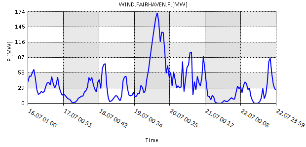
plot('WIND.FAIRHAVEN.P.[MW]')-
The plot function uses an expression to chart the power generated by the wind generator FAIRHAVEN within the time properties defined
ChartStartTimeandChartEndTime.
2. Special parameters in expressions
You may have noticed that in the examples of the previous section, there are some expressions with some extra characters. SAInt allows the user to easily extend the meaning of an object expression by adding special parameters. The general syntax for using these special parameters is:
ObjectType.%.PropertyExtension.[Unit].(%)/(Time)
where:
%
|
The symbol |
[Unit]
|
The unit of measure is an optional special parameter. If no unit information is specified, then the property value will be displayed in the unit specified for the corresponding unit type and property of the general settings. If a different unit is specified, SAInt takes care of the conversion. For example, 'WIND.%.P.[MW]` indicates that the total power of the wind generators is expressed in megawatt. The units can be changed in the units tab under SAInt GUI settings. |
(%) or (Time)
|
The time definition is optional. In its general form |
Another case is:
ObjectType.!ObjectType
where:
!
|
The exclamation mark symbol is used in an input expression containing a two-level nested hierarchy of object types. The symbol goes before the second type which is a child of the first. When we type |
2.1. Arithmetic expression
Arithmetic expressions allow to combine object expressions using mathematical operations such as addition, subtraction, multiplication, square root, cosine, sine, logarithm, etc. An arithmetic expression can take as arguments only network parameters (i.e., object expressions for properties) or mix network parameters and numerical constants. Check the List of available mathematical functions. for more details.
The eval function must be used to compute the value of an arithmetic expression. The function eval accepts as arguments: an object expression for a property or mathematical combinations of object expressions for a property and numerical constants. It always returns a numeric value. This result can be further used as input for other IronPython arithmetical functions.
List of available mathematical functions.
| Function | Description |
|---|---|
|
The function returns the integer part of x with the fractional part removed. |
|
The function returns the arc cosine (inverse cosine) of a number in radians. |
|
The function returns the inverse hyperboilic cosine of a number in radians. |
|
The function returns the cosine of the given angle. |
|
The function returns the hyperbolic cosine of a number in radians. |
|
The function returns the arc sine (inverse sine) of a number in radians. |
|
The function returns the inverse hyperboilic sine of a number in radians. |
|
The function returns the sine of the given angle. |
|
Returns the hyperbolic sine of a number in radians. |
|
The function returns the arc tan (inverse tan) of a number in radians. |
|
The function returns the arctangent, or inverse tangent, of the specified x- and y-coordinates. |
|
The function returns the hyperboilic tan of a number in radians. |
|
The function returns the tangent of the given angle. |
|
The function returns the hyperbolic tangent of a number in radians. |
|
The function returns the angle (radian) in degrees. |
|
Natural exponential function. |
|
The function returns the factorial of a number. |
|
The function returns the natural logarithm (Base e) of a number. |
|
The function returns the base-10 logarithm of a number. |
|
The function returns the natural logarithm (base e) of 1 + p, where p is the argument. |
|
The function returns the value of the mathematical constant PI ~ 3.14159. |
|
The function returns the value of the mathematical constant e ~ 2.71828182845905. |
|
The function returns the angle (degrees) in radians. |
|
The function returns the square root of a number. |
|
The function returns the mean of a list of float values. |
|
The function returns the ceiling of the variable as a float and the smallest integer value greater than or equal to the variable. |
|
The function returns a variable x with the sign of a second variable y. |
|
The function returns the error function value as a float at the variable. |
|
The function returns the complementary error function value as a float at the variable. |
|
The function returns the natural exponential function minus one for small float values. |
|
The function returns the absolute value of a variable. |
|
The function returns the floor of a variable x as a float, the largest integer value less than or equal to the variable x. |
|
The function returns the modulo, the remanent after the division, of varible x by another variable y. |
|
The function returns the mantissa and exponent of x as the pair (m, e). m is a float and e is an integer such that x == m * 2**e exactly. If x is zero, returns (0.0, 0), otherwise 0.5 ⇐ abs(m) < 1. This is used to “pick apart” the internal representation of a float in a portable way. |
|
The function returns an accurate floating point sum of values in list. |
|
The function returns x*2y. It is the inverse of function |
|
The function returns the Gamma function at the variable. |
|
The function returns a natural logarithm of the absolute value of the Gamma function at the variable. |
|
The function returns the Euclidean norm, sqrt(x*x + y*y). This is the length of the vector from the origin to point (x, y). |
|
The function returns the fractional and integer parts of a variable x. Both results carry the sign of the variable x and are floats. |
|
The function returns a variable x raised to the power of another variable y. |
ENET.PG.(10).[GW]-
This is a regular object expression and not an arithmetic expression. It returns a value of type string, even if we see numerical digits.
eval('ENET.PG.(10).[GW] + 5')-
This is the correct way of combining an object expression for a property and a constant with the same units. The evaluation function returns the sum of active power generated by the electric network at the 10th hour of the simulation in megawatt and a constant value of 5 megawatt.
eval('ENO.HARTFORD_CT.PPV.[MW].(%) * 10')-
The expression returns a list with the values of the active power in megawatt generated by all solar generators connected to the electric node HARTFORD_CT during all time steps of the simulation. Each time step value is multiplied by 10. In the example, we have only one solar generator associated with HARTFORD_CT.
eval('GDEM.CITY1.Q.[ksm3/h].(3) + GDEM.INDUSTRY3.Q.[ksm3/h].(3)')-
The arithmetic expression returns the sum in ksm3/h of the demand of the externals GDEM.CITY1 and GDEM.INDUSTRY3 at the 3rd hour of the simulation. The value is 308 ksm3/h.
eval('sqrt(ENET.PG.[MW].(5))')-
Returns the square root of the power generated by the electric network at the 5th hour of the simulation.
|
Check the content of the workspace in SAInt for a list of mathematical functions. |
|
2.2. Conditional expression
Conditional expressions allow to use of Boolean algebra in expressions, and in their most basic form to check whether a statement is true or false. The conditional expression can combine different network parameters, arithmetic expressions, or constant values. The expression returns Boolean "True" or "False" values. As for arithmetic expressions, a conditional expression must be used as argument to the eval function.
eval('FGEN.SIMONDS.P.(%).[MW] >= FGEN.SIMONDS.PMIN.(%).[MW]')-
Checks if the power generated by the fuel generator SIMONDS is greater or equal to its minimum power generation (
PMIN) at each time step and returns a list of true or false values. The length of the list is equal to the number of time steps in the simulation. eval('ENET.PG.(10).[GW] > 5')-
Checks if the active power generation by the electric network is greater than 10 GW at the 10th hour of the simulation and returns a true or false value.
eval('FGEN.SIMONDS.P.[MW].(%) > 80 and FGEN.SIMONDS.P.[MW].(%) < 150')-
The expression checks if the power generated by the fuel generator SIMONDS is between 80 MW and 150 MW at each time step of the simulation and returns a list of true or false values. The length of the list equals the number of time steps in the simulation.
eval('GDEM.CITY1.Q.[ksm3/h].(3) > GDEM.INDUSTRY3.Q.[ksm3/h].(3)')-
The expression checks if the demand flow at the external GDEM.CITY1 is higher than the one at the external GDEM.INDUSTRY3 at the 3rd hour of the simulation. The answer is False.
|
Only a single network parameter can be used for combined conditional expressions (Object Type, Object ID, and Property Extension must be the same). |
2.3. Control value expression
Control value expressions are special and optional expressions used with plotting functions such as nplot or stackplot. They are very useful in charts because they allow to add reference values like a constant line representing a threshold or a desired value to reach. Control value expression cannot be used as a stand-alone expression, but must be used with some other object expressions. Furthermore, it is necessary to specify the unit of measure used like 70[MW].
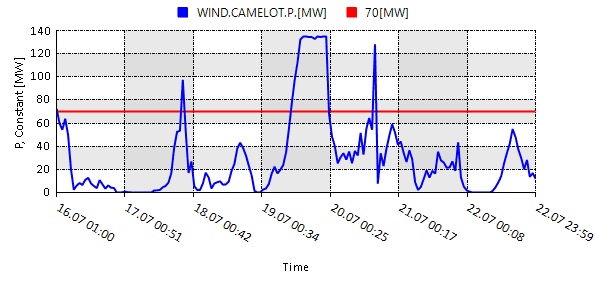
nplot('WIND.CAMELOT.P.[MW];[140;0;7];Blue','70[MW];Red')-
Plots the power generated by the wind generator CAMELOT and a control value of 70 MW.
2.4. Time expression
Time expressions are used in time-dependent functions to indicate either the exact time step to be used or to define the time window considered. Examples of time-dependent functions are the time function or the different functions for plotting or creating tables.
If any time expression is specified, the default behavior of the time-dependent functions is to use the default start time and end time given by the ChartStartTime and ChartEndTime properties in the scenario editor.
Time expressions are always a string type and not numeric values. This explains why they must be between quotation marks.
When the time is explicitly indicated, the format must match the one set for date and time in the general settings of SAInt, check the property DateTimeFormat in the section "Miscellaneous".
The function time() uses a sophisticated syntax to specify how to add or set time. The user can write:
-
+nwherenis an integer indicating the number of hours to add to the active time. -
-nwherenis an integer indicating the number of hours to be used to reset the time. Ifnis in [0;24], the function resets the time to the specified hour (using the 24-hour notation) for the same day. Ifnis bigger than 24, the function will first move the day ahead with steps of 24 hours, and then reset the time for the new day to the difference between the originalnand the number of 24-hour steps. For example,-37adds one day and sets the time to 13:00 (or 1 p.m.). -
+X.Y:ZwhereXis an integer indicating the number of days to add,Yis an integer indicating the number of hours to add, andZis an integer indicating the number of minutes to add. -
-X.Y:ZwhereXis an integer indicating the number of days to add,Yis an integer indicating the hour to set, andZis an integer indicating the value of the minutes to set.
time('+1')-
Increase the time of the map window by one hour.
time('-1')-
Reset the time of the map window to 01:00 of the active day.
time('+1.1:05')-
Increase the time of the map window by one day, one hour and five minutes.
time('-1.1:15')-
Reset the time of the map window to 01:15 after adding one day.
time('20/07/2023 23:00')-
The resulting display time on the map window is 20-July-2023 23:00.
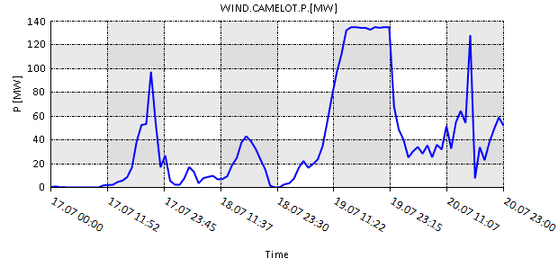
plot('WIND.CAMELOT.P.[MW];[140;0;7];Blue','17/07/2023 00:00','20/07/2023 23:00')-
Plots the power generated by the wind generator CAMELOT for the defined time window (17-July-2023 00:00 until 20-July-2023 23:00). -
2.5. Time record
After a non-steady simulation, like dynamic gas or QuasiDynamicACPF, SAInt records the simulation time into the workspace with time record functions in hours as numeric expressions, either as floats or a list of floats. Check the List of time record functions..
List of time record functions.
| Function | Description |
|---|---|
|
Returns a list of float values, a record of all time steps in the electric simulation. |
|
Returns a list of float values, a record of all time steps in the gas simulation. |
|
Stores the float value of the time step of an electric simulation as it progresses in time, it makes the time step callable in expressions and functions. |
|
Stores the float value of the time step of a gas simulation as it progresses in time, it makes the time step callable in expressions and functions. |
|
Returns the float value of the electric simulation time step, equivalent to the |
|
Returns the float value of the electric simulation time step, equivalent to the |
|
Returns the float value of the last record in |
|
Returns the float value of the last record in |
print(gtimes)-
Prints in the command window all the time steps of the scenario BAU_DYNAMIC.gsce, from 0.0 to 72.0 in increments of 0.25 h.
gtmax-
Returns
72equal to theTimeWindowof BAU_DYNAMIC.gsce. gdt-
Returns
0.25equal to theTimeStepof BAU_DYNAMIC.gsce.