Step 1: Create a Coupled Gas-Electric Networks Model

Your first step in this intermediate-level tutorial aims at creating a simple coupled gas-electric networks model for a combined dynamic simulation over three days. The coupled model is comprised of:

five pipelines, two supply points, a compressor station, and five demand points in the gas system;
five high-voltage lines, three demand points, two generic generators, and one wind farm in the electric system;
and two coupling points: an electric-driven compressor station and a power-to-gas facility with an electrolyzer producing hydrogen.

1. Create a new project and add your networks

Let’s start the tutorial by creating a new empty project. Save it with the name coupled in its own directory. Please, revise the units of measure, as the tutorial uses units based on the International System and euro as currency.

You can now add to your project the two single-carrier energy networks you want to analyze together in an exercise of combined simulation.

1.1. The gas network

As for the gas system, you will use the same gas model created for the first intermediate-level tutorial for gas networks, with minor changes. You can find a copy of the system in the tutorial’s directory, in the sub-folder .\Coupled\Intermediate Tutorial 1\Initial.

Decompress the archive and save the directory gNetwork1 inside the directory coupled. Now open the gas network gNetwork1 from the GUI. SAInt will load the system and display it in a map view window.

You can read more about this system in "Step 1: Create a Gas Network Model" of the intermediate-level tutorial on gas networks covering contingencies and hydrogen blending. But, in a nut-shell the system (Figure 1) has:

a leading supply point importing gas of quality IMPORT composed of methane and ethane at a pressure of 45 bar-g;
a gas-driven compressor station with a fixed POSET control mode equal to 48 bar-g, the property ExtractFuel is TRUE, and the efficiencies are set as EFFHDEF equal to 0.78 and EFFMDEF equal to 0.7;
a second supply point P2H2 modeling an electrolyzer injecting small volumes of pure hydrogen (i.e., the gas quality Hydrogen with 100 % in molar mass of H₂);
two demand objects describing households consumers (i.e., objects GDEM.CITY1 and GDEM.CITY2) linked to nodes with a minimum delivery pressure of 5 bar-g (i.e., PMINDEF equal 5 bar-g and PMINPRCDEF set to 100 €/bar);
three demand objects describing industrial users, with the external GDEM.INDUSTRY1 linked to a node with a minimum delivery pressure of 5 bar-g, the external GDEM.INDUSTRY2 linked to a node with a minimum delivery pressure of 27 bar-g and the external GDEM.INDUSTRY3 to a node at 25 bar-g;
the total network length is 180 kilometers;
quality tracking is active;
temperature tracking is active, with all supply sources set to 15 °C, overall network ambient temperature at 5 °C, and the pipeline PIPE4 at 0 °C.

Check the properties of the network object gNetwork1 and ensure the reference temperature (Tn) equal to 0 °C and the reference pressure (Pn) equal to 1.01325 bar. In this way, you assume to use the so-called "normal condition" of the standard LST EN ISO 13443.

The model has one steady state reference scenario and three dynamic scenarios. The first dynamic scenario BAU_DYNAMIC, models a business-as-usual case. The second scenario, S1_DYNAMIC, models a contingency on the main supply point. The third scenario, H2_DYNAMIC, studies how to increase the electrolyzer’s use while coping with downstream users' constraints on the quality of the delivered gas mixture.

All dynamic scenarios use profiles with hourly time steps covering three days (i.e., 72 hours). The first and the last day are equal, while the second day has higher values representing peak conditions.

Please, take some time to familiarize yourself with the model by running all scenarios and exploring the behavior of the compressor station, demand off-take INDUSTRY2 and INDUSTRY3. Alternatively, you could pause here and take some time to review the intermediate-level gas network tutorial.

Remember to save your project before moving on.

Figure 1. Diagram of the gas network used in the tutorial.

In Figure 1, under the node name, the location is expressed with coordinates in kilometers (e.g., node N2 is at x 25 km and y 0 km). The node color follows SAInt convention: green for supply, red for demand, orange for mixed, and light grey for nodes without externals. The icon t01 step01 021 indicates that the node has an associated external of type demand. The icon t01 step01 022 indicates a supply. The pipeline length is not in scale.

1.2. The electric network

As for the electric system, you will use a simple electric network as described in Figure 2. The network is comprised of five high-voltage lines, three demand points, two generic generators, and one wind farm. You can find a copy of the system in the tutorial’s directory, in the sub-folder .\Coupled\Intermediate Tutorial 1\Initial.

You can either build the network by using the details provided below or you can find a copy of the network in the tutorial’s directory.

Figure 2. Diagram of the electric network used in the tutorial.

In Figure 2, under the node name, the location is expressed with coordinates in kilometers (e.g., node N1 is at x 0 km and y -30 km). The node follows SAInt convention: green for supply and red for demand. The icon t01 step01 031 indicates that the node has an associated external of type demand. The icon t01 step01 032 indicates a wind farm, while the icon t01 step01 033 is a generic generator. The electric line length is not in scale.

The following tables provide the details needed to complete the network. Default values are assumed for all details not presented in the tables.

Click here to view the properties of the nodes of the tutorial electric network.

Table 1. Data for the node objects. The extended name and the extension of the object are reported to facilitate the editing. Extensions in bold are mandatory.
Object Name	Normal voltage magnitude	Default maximum voltage magnitude	Default minimum voltage magnitude
`Name`	`BaseV`	`VMAXDEF`	`VMINDEF`
N1	230 [kV]	1.05 [pu]	0.95 [pu]
N2	230 [kV]	1.05 [pu]	0.95 [pu]
N3	230 [kV]	1.05 [pu]	0.95 [pu]
N4	230 [kV]	1.05 [pu]	0.95 [pu]
N5	230 [kV]	1.05 [pu]	0.95 [pu]

Click here to view the properties of the electric lines.

Table 2. Data for the electric line objects. The extended name and the extension of the object are reported to facilitate the editing. Extensions in bold are mandatory.
Object Name	Default maximum current magnitude	Default maximum apparent power	Line resistance per length	Line reactance per length	Total length of the electric line	Calculate Impedances
`Name`	`IMAXDEF`	`SMAXDEF`	`RRL`	`XXL`	`L`	`CalcImp`
LI1	1150 [A]	250 [MVA]	0.042 [Ω/km]	0.275 [Ω/km]	100.0 [km]	TRUE
LI2	1150 [A]	250 [MVA]	0.042 [Ω/km]	0.275 [Ω/km]	50.0 [km]	TRUE
LI3	1150 [A]	250 [MVA]	0.042 [Ω/km]	0.275 [Ω/km]	100.0 [km]	TRUE
LI4	1150 [A]	250 [MVA]	0.042 [Ω/km]	0.275 [Ω/km]	50.0 [km]	TRUE
LI5	1150 [A]	250 [MVA]	0.042 [Ω/km]	0.275 [Ω/km]	50.0 [km]	TRUE

Click here to view the properties of the electric demand objects.

Table 3. Data for the electric demand objects. The extended name and the extension of the object are reported to facilitate the editing. Extensions in bold are mandatory.
Object Name	Node Name	Default maximum active power	Power factor	Power factor type	Default penalty price for minimum active power
`Name`	`NodeName`	`PMAXDEF`	`PWF`	`PWFType`	`PMINPRCDEF`
CS1	N4	8.00 [MW]	0.85 [-]	ind	0 [€/MWh]
DEM1	N4	400.00 [MW]	0.85 [-]	ind	0 [€/MWh]
P2H2	N4	54.53 [MW]	0.97 [-]	ind	0 [€/MWh]

Click here to view the properties of the generic generator objects.

Table 4. Data for the generic generator objects. The extended name and the extension of the object are reported to facilitate the editing. Extensions in bold are mandatory.
Object Name	Node Name	Default maximum active power	Default minimum active power	Default active power slack participation factor	Default voltage magnitude set point	Default maximum reactive power	Default minimun reactive power
`Name`	`NodeName`	`PMAXDEF`	`PMINDEF`	`PFSETDEF`	`VMSETDEF`	`QMAXDEF`	`QMINDEF`
XGEN1	N3	110 [MW]	0 [MW]	20 [-]	1.01 [pu]	160 [MVAr]	-160 [MVAr]
XGEN2	N1	250 [MW]	100 [MW]	80 [-]	1.03 [pu]	200 [MVAr]	-200 [MVAr]

Click here to view the properties of the wind farm object.

Table 5. Data for the wind farm object. The extended name and the extension of the object are reported to facilitate the editing. Extensions in bold are mandatory.
Object Name	Node Name	Default maximum active power	Default penalty price for minimum active power	Latitude	Longitude
`Name`	`NodeName`	`PMAXDEF`	`PMINPRCDEF`	`Lat`	`Long`
WIND_FARM	N5	80 [MW]	0 [€/MWh]	46.8976 [-]	-96.9031 [-]

Total system losses Name of the wind turbine power curve Hub height of the wind generator

Total system losses	Name of the wind turbine power curve	Hub height of the wind generator
`LOSSES`	`WTPCName`	`HubHeight`
14.1 [%]	COMPOSITE_CLASS_II	84 [m]

LOSSES

WTPCName

HubHeight

14.1 [%]

COMPOSITE_CLASS_II

84 [m]

This simple electric model does not incorporate meteorological wind speed data for the wind generator WIND.WIND_FARM. However, the wind turbine power curve (COMPOSITE_IEC_CLASS_II), hub height, and longitude and latitude give you all the basic elements to take this extra step. Check the section of the reference guide Integrating Weather Resource Data for more details, or try the How-To Create a Wind Generation Profile with Weather Data for a practical introduction to the topic.

Revise the properties of the network object eNetwork1 and the units of measure to ensure everything is clear and fits your needs.

The model has one reference steady state ACPF scenario Steady_ACPF and one quasi-dynamic ACPF scenario QuasiDynamic_ACPF. The set of events of the steady state simulation is presented in Table 6. Take the time to check the events and run the simulation just for this system.

Notice how SAInt expects you to fully specify the simulation problem by providing all relevant constraints for supply and demand for all the externals. When running a combined simulation, this is not necessary, as conditions on one system explicitly define constraints on the other.

Table 6. Data for the steady state ACPF scenario **Steady_ACPF** of the tutorial electric network.
Object Name	Parameter	Value	Unit of Measure
WIND_FARM	`PSET`	50.0	MW
WIND_FARM	`QSET`	0.0	MVAr
XGEN1	`PSET`	50.0	MW
XGEN2	`PSET`	150.0	MW
DEM1	`PSET`	250.0	MW
P2H2	`PSET`	54.5	MW
CS1	`PSET`	8.0	MW

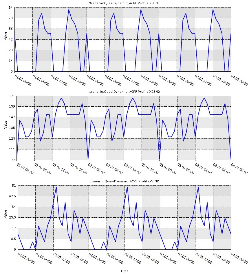
The set of events of the quasi-dynamic ACPF QuasiDynamic_ACPF simulation is presented in Table 7. Take your time to understand the events, mainly the conditions for the two generic generators. The generator XGEN2 operates by always providing active power to the system. Its slack participation factor changes by following the value of PSET for the time step.

The generator XGEN1 operates similarly, but it turns on or off based on the value of its profile. When the profile goes to zero, the generator goes off, which is a technique to avoid manually adding many events to the service! Look at Figure 3, which shows the profiles of the generators.

Table 7. Data for the quasi-dynamic ACPF scenario **QuasiDynamic_ACPF** of the tutorial electric network.
Start Time	Object Name	Parameter	Profile	Condition	Evaluation	Value	Unit of Measure
01/02/2020 00:00	WIND_FARM	`PSET`	WIND		NONE	1.0	MW
01/02/2020 00:00	WIND_FARM	`QSET`			NONE	1.0	MVAr
01/02/2020 00:00	DEM1	`PSET`	DEM1		NONE	1.0	MW
01/02/2020 00:00	P2H2	`PSET`			NONE	35.44	MW
01/02/2020 00:00	CS1	`PSET`			NONE	8.0	MW
01/02/2020 00:00	XGEN1	`PSET`	XGEN1		NONE	1.0	MW
01/02/2020 00:00	XGEN1	`PFSET`			NONE	XGEN.XGEN1.PSET	-
01/02/2020 00:00	XGEN1	`OFF`		XGEN.XGEN1==0	DoIFTRUE
01/02/2020 00:00	XGEN1	`ON`		XGEN.XGEN1>0	DoIFTRUE
01/02/2020 00:00	XGEN2	`PSET`	XGEN2		NONE	1.0	MW
01/02/2020 00:00	XGEN2	`PFSET`			NONE	XGEN.XGEN2.PSET	-

Figure 3. Profiles for the two generic generators and for the wind farm generator in the tutorial network.

The value of an event can be an expression that SAInt needs to evaluate and not just a fixed number. See the case for the events PFSET XGEN1 and XGEN2. The events depend on the objects' PSET value; the last depends on their correspondent objects' event profile.

Profiles in QuasiDynamic_ACPF are absolute, while they are relative in any of the gas scenarios. Absolute profiles require an event with a magnitude equal to one. Relative profiles have values indicating the proportions of the event value.

If you are rebuilding from scratch the electric network, add profiles by including the file that you can copy from the tutorial’s directory. Select Data>Include>Profile(s) To Electric Scenario (ESCE) from the Scenario tab and specify the location of the file. A message will inform that the profiles have been correctly included in the scenario.

Finally, note that on the demand side, the scenario specifies a profile just for the external DEM1. Assume the electric demand in CS1, an electric-driven compressor station, and in P2H2, an electrolyzer, are at a near peak during the simulation.

Before moving to the next section, please save your project.

2. Create a coupled networks model using HUBS

When dealing with coupled models, you need to take a few extra steps before running a combined simulation. The first of these extra steps is to create a "hub system" (HUBS object). The hub system is a particular type of "network". As with any other network, it is composed of objects representing nodes in a graph and of links describing branches. A node in the hub system is made up of objects belonging to single energy-carrier networks. A link in the hub system is a coupling relationship between such original objects, and it describes how networks interact at those points.

For example, you can picture a hub system object, like an electric-driven compressor station (EDGCS object), as a gas object "compressor station" (GCS) and an electric external "demand of electricity for the compressor station" (EDEM.GCS) linked by a coupling relationship describing how much electric power is needed to operate the compressor.

Check the section hub objects of the reference guide for an extensive description of the objects and properties for creating and modeling hub systems.

Creating a "hub system" (HUBS object) requires:

First step	Load participating networks Load the single-energy networks contributing to the coupled model in the active project. Use the options File>Open Open Gas Network and File>Open Open Electric Network from the Network tab to load your existing models. Alternatively, you may create the models from scratch. You may organize your SAInt session as you wish, but having a map view tab showing only the gas network and a second map view showing only the electric network is helpful.
Second step	Create a hub system object Select File>New New Hub System from the Network tab. SAInt will ask for a directory where to save the new object and its associated files. Create a new folder named HUBS inside the project directory coupled. A new hub system object HUBS is available in the model explorer. New files are created in the directory HUBS. Use a third map view tab to display the hub system and the gas and electric network. Ensure that all three elements are ticked in the drop-down list at the top-right of your map view window. Because there is no coupling object, nothing special is shown for the hub system.
Third step	Create coupling objects Populate the hub system by specifying which objects from the participating networks define the coupling relationships. Select the compressor station GCS.CS1 in the model explorer of the gas network gNetwork1. Right-click and, from the context menu, select Add New Hub Electric-Driven Gas Compressor. SAInt shows a list of possible coupling links. Choose the one saying EDEM.CS1 <-> GCS.CS1. Congratulation! You have just created your first coupling relationship. You can find the new object in the model explorer under the HUBS branch in HubFacilities. A second approach is to use the map view. Select the node ENO.N2 in the map view where the hub system is displayed. Right-click and, in the context menu, select Add New Hub Power-To-Gas Facility. SAInt shows a list of possible coupling links. Choose the one saying EDEM.P2H2 <-> GSUP.P2H2.

SAInt represents coupling entities in the map view using a dashed cyan line linking the contributing objects. You can add labels to the line or access the link properties by double-clicking after selecting it using the context menu and choosing the property editor.

Remember to activate the class HUBS in the map view to show the coupling links.

Fourth step

Edit the properties of the coupling objects

The last step in setting up a hub system is to edit the properties of the coupling objects.

Open the property editor for the electric-driven compressor station from the context menu using either the model explorer or the link in the map view tab. Change the object name from the property editor window into HUB_CS1. Make sure that the power factor (PWF) is equal to 0.85 and the power factor type (PWFType) to "ind".

Now select GCS.CS1 from the map view or the model explorer and open the property editor for the gas object. Change the mechanical efficiency (EFFMDEF) to 0.80, and deselect the option to extract fuel ('ExtractFuel'). This last step helps keep your model well organized. When a gas-driven compressor is part of a coupling object, SAInt does not consider the extraction of gas fuel even if the option is TRUE.

Move to the power-to-gas facility, and from the property editor, change the name to HUB_P2H2. Make sure that the power factor (PWF) is equal to 0.97 and the power factor type (PWFType) is "ind". Change the efficiency factor for the power-to-gas conversion ('Eff') to 0.65.

You have finished setting up the coupling objects EDGCS.HUB_CS1 and P2G.HUB_P2H2, and to edit their properties. You are now ready to create a new scenario for a combined simulation.

Before proceeding, remember to save your project.

You may add labels to the coupling links in the map view as an additional activity. For EDGCS.HUB_CS1 you could use the properties Name, POWD, and PD for displaying the name, the driver power and the active power consumed. For P2G.HUB_P2H2 you could use in the properties Name, PD, and Q for displaying the name, the active power, and the hydrogen flow injected in the network.