Step 1: Create a Gas Network Model
In this tutorial, you start by creating a simple gas model used to carry out a dynamic simulation over three days. The gas model has five pipelines, two supply points, a compressor station, and five demand points. The model considers two different streams of gases and temperature tracking.
1. Create a new project and build your network
You have learned the basics of drawing your network in the beginner tutorials. Now it is time to put into good practice your knowledge. The main advantage of building your system directly in the SAInt GUI is that you take the time to define all relevant details of the nodes, the branches, and the externals. Furthermore, topological consistency is immediately enforced. For simple projects, this approach is fantastic!
For more complex networks, manually drawing can be time-consuming. A better strategy would be to use templates in Excel™ or shapefile format to quickly organize your data and then take advantage of SAInt’s import capabilities.
1.1. Create a new project
The first thing you need to do is to create a new empty project and select the basic properties of your model. The project stores the model and its data, scenarios, results, and simulation scripts. The project settings will address some fundamental aspects like units of measure, reference conditions, or type of equation used for friction or compressibility.
When launching the SAInt GUI, you see the default "New Project" space. Click on  and select Save Project. Please create a new folder named Intermediate1GNET and select it. The project is renamed out of the folder and saved there.
Now, select again and go to Settings. In the new window, select "Units" tab and specify the set of units of measure and the currency you prefer. In the tutorial, you will use commonly applied units from the International System and the euro as currency. For example, you could change the XY-Coordinate from kilometers to meters. Remember to click on Apply!
1.2. Draw the tutorial network
Now that your project is ready, it is time to start creating your network. Go to the Network tab and select . Create a new directory named gNetwork1 inside the project folder and click Select Folder. A new simple network is generated.
Following, from the model explorer, select the entry GasNetwork - (gNetwork1) under Networks and check the properties in the property editor. If not already open, right-click and select menu:[open Editor] from the context menu to access the property editor. From there, you may change fundamental aspects of your model, like the compressibility factor equation (you stick with the default PAPAY) or the friction factor equation (keep Hofer). Make sure to have the reference temperature (Tn) equal to 0 °C and the reference pressure (Pn) at 1.01325 bar. In this way, you assume to use the so-called "normal condition" of the standard LST EN ISO 13443.
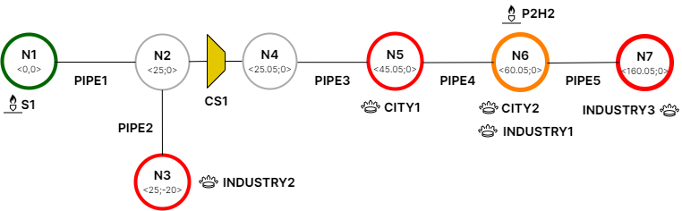
Use the information in Figure 1 to draw the tutorial network. Start by changing the name of the two nodes: GNO_0 should be N1, and GNO_1 should be N2. Select node GNO.N2 now and, from the property editor, adjust its X-Coordinate (property X) to 25 km and Y-Coordinate (Y) to 0 km. Change the Name of the pipe GPI_0 to PIPE1. Then, update its length (L) to 25 km. Continue by adding the new pipelines and the compressor station. Complete the system’s geometry and topology by updating the nodes' names.
Once the network is complete, it is time to add the externals. Follow the scheme in Figure 1 and add the supply or demand objects with the correct name to each node.
|
In Figure 1 under the node name, the location is expressed with coordinates in kilometers (e.g., node N2 is at x 25 km and y 0 km). The node color follows SAInt convention: green for supply, red for demand, orange for mixed, and light grey for nodes without externals. The icon |


1.3. Edit objects properties
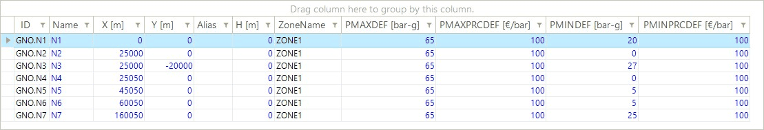
Use "tables" to quickly edit the objects' properties you just have created. For example, from the Table tab of the SAInt GUI select  to open the table of nodes of the model. You can arrange or hide the existing columns and show new columns with the option "Show Column Chooser" by right-clicking in the blank space below the table. Figure 2 shows an example of the possible layout of the table. Edit the properties of the nodes using the data provided in Table 1. Leave the default value for all other properties not mentioned in the table.
Click here to view the properties of the nodes of the tutorial network.
| Object Name | Default maximum pressure | Default penalty price for maximum pressure | Default minimum pressure | Default penalty price for minimum pressure |
|---|---|---|---|---|
|
|
|
|
|
N1 |
65 [bar-g] |
100 [ |
20 [bar-g] |
100 [ |
N2 |
65 [bar-g] |
100 [ |
0 [bar-g] |
100 [ |
N3 |
65 [bar-g] |
100 [ |
27 [bar-g] |
100 [ |
N4 |
65 [bar-g] |
100 [ |
0 [bar-g] |
100 [ |
N5 |
65 [bar-g] |
100 [ |
5 [bar-g] |
100 [ |
N6 |
65 [bar-g] |
100 [ |
5 [bar-g] |
100 [ |
N7 |
65 [bar-g] |
100 [ |
25 [bar-g] |
100 [ |
Follow the same approach for the pipelines and the compressor station. Start by opening the table for that object type, then adjust its columns and edit the properties. For pipelines, use the data provided in Table 2. For the compressor station, use the data in Table 3.
Click here to view the properties of the pipelines of the tutorial network.
| Object Name | Inner Pipe Diameter | Pipeline Efficiency | Pipeline Length | Inner Wall Roughness of the Pipeline | Thickness of the Pipeline Wall |
|---|---|---|---|---|---|
|
|
|
|
|
|
PIPE1 |
482.6 [mm] |
1 |
25 [km] |
0.012 [mm] |
12.7 [mm] |
PIPE2 |
431.8 [mm] |
1 |
20 [km] |
0.012 [mm] |
12.7 [mm] |
PIPE3 |
482.6 [mm] |
1 |
20 [km] |
0.012 [mm] |
12.7 [mm] |
PIPE4 |
431.8 [mm] |
1 |
15 [km] |
0.024 [mm] |
12.7 [mm] |
PIPE5 |
431.8 [mm] |
1 |
100 [km] |
0.024 [mm] |
12.7 [mm] |
Click here to view the properties of the compressor station branch of the tutorial network.
| Object Name | Design Diameter of non-Pipelie Bracnhes | Deafault Average Adiabatic Efficiency | Default Average Driver Efficiency | Default Minimum Inlet Pressure | Default Penality Price for Minimum Inlet Pressure |
|---|---|---|---|---|---|
|
|
|
|
|
|
CS1 |
482.6 [mm] |
0.78 |
0.7 |
10 [bar-g] |
100 [€/bar] |
| Default Maximum Outlet Pressure | Default Penality Price for Maximum Outlet Pressure | Default Maximum Driver Power | Default Penality Price for Maximum Driver Power | Default Maximum Shaft Power | Default Penality Price for Maximum Shaft Power |
|---|---|---|---|---|---|
|
|
|
|
|
|
60 [bar-g] |
100 [€/bar] |
8 [MW] |
100 [€/MWh] |
5.5 [MW] |
100 [€/MWh] |
| Default Maximum Pressure Ratio | Default Penality Price for Maximum Pressure Ratio | Default Maximum Flow Rate | Default Penality Price for Flow Rate |
|---|---|---|---|
|
|
|
|
1.6 |
100 [€] |
3000 [ksm3/h] |
100 [€/sm3] |
| Default Maximum Volumetric Flow Rate | Default Penality Price for Maximum Volumetric Flow Rate | Default Maximum Flow Velocity | Default Penality Price for Maximum Flow Velocity | Extract Required Fuel from Inlent Node |
|---|---|---|---|---|
|
|
|
|
|
100 [m3/s] |
100 [€/m3] |
60 [m/s] |
100 [€/m] |
TRUE |
You are almost there! Now it is time to edit the externals. Go ahead and use the data provided in Table 4 and Table 5 to complete the gas supply and the gas demand externals.
Click here to view the properties of the supply externals of the tutorial network.
| Object Name | Node Name | Default maximum outflow | Default penalty price for maximum outflow | Name of scheduled supply gas quality |
|---|---|---|---|---|
|
|
|
|
|
S1 |
N1 |
450 [ksm3/h] |
100 [€/sm3] |
DEFAULT |
H2FEED |
N6 |
10 [ksm3/h] |
100 [€/sm3] |
DEFAULT |
Click here to view the properties of the demand externals of the tutorial network.
| Object Name | Node Name | Alternative Object Name | Information Entered fo the Object | Default maximum inflow | Default penalty price for maximum inflow |
|---|---|---|---|---|---|
|
|
|
|
|
|
CITY1 |
N5 |
Essen |
City Gate |
75 [ksm3/h] |
100 [€/sm3] |
CITY2 |
N6 |
Denver |
City Gate |
75 [ksm3/h] |
100 [€/sm3] |
INDUSTRY1 |
N6 |
Tyrell Corp. |
Industry |
100 [ksm3/h] |
100 [€/sm3] |
INDUSTRY2 |
N3 |
ACME Inc. |
Industry |
150 [ksm3/h] |
100 [€/sm3] |
INDUSTRY3 |
N7 |
Oscorp |
Industry |
200 [ksm3/h] |
100 [€/sm3] |
|
Remember to save your network and your project from time to time. |
1.4. Use a template
Indeed, the most significant advantage of creating your network directly in SAInt is that you have complete control of all steps. When building your network in the GUI, you double-check the objects' properties and details or customize your project immediately. But this scales up with the size of your network! And when you go big, you may be looking for alternatives to create your model and transfer the data.
SAInt allows for importing networks and data in alternative ways. You can use Excel templates to easily collect and organize data from multiple sources in a simple table layout.
Look at the files in C:\...\Documents\encoord\SAInt-v3\DataImport to find the templates. Check the section data exchange for an in-depth description of the templates' structure, mandatory fields, data organization, and procedures for importing.
You can use the Excel template attached to this intermediate tutorial.
Copy the network data Excel file "gnetwork1.xlsx" from the sub-folder .\Gas Networks\Intermediate Tutorial 1 of the folder Tutorials in the directory (C:\Users\...\Documents\encoord\SAInt-v3\Projects). Save it in your project directory and select from the Network tab. The import procedure will ask for the Excel template, the name, and the location of the new network. A message will inform you of the successful import, indicating the number of nodes and branches imported. The new network is available in the active project, and you are ready to go.
|
Try to create your own version of the template. Start with an empty one and use the previous section’s nodes, branches, and externals details to fill the template in. This is a good exercise to understand how templates work. |