Step 4: Build a DCUCOPF Scenario

In the previous steps of this tutorial, you created an electric power system represented by a triangular network. This step will focus on creating a production cost model, referred to as Direct Current-approximation Unit Commit Optimal Power Flow (DCUCOPF) in SAInt. You will create an optimization scenario for the day-ahead market operation of the power system based on daily optimizations and hourly timesteps. The objective is to learn how to create a scenario in SAInt and how different parameters affect the behavior of the scenario.

Before starting this tutorial, follow the steps below to open the previously created network.

Go to the network tab and click on Open Open Electric Network option.
Use the navigation window to locate the project folder C:...\Documents\encoord\SAInt-v3\Projects\Tutorial_ENETs.
Select the file Tutorial_ENET.enet and click on Open to load the network file in SAInt.

1. Create a new scenario

Create a new scenario by going to the scenario tab and selecting New New Electric Network Scenario. This will open the scenario dialog window. Here, you will define the parameters and settings of the scenario. The first step is to define the scenario type in the top left corner under 1. Select Scenario Type click on the drop-down menu and select DCUCOPF. Under the 2. Enter Scenario Name type DCUCOPF_5Day as shown in Figure 1. The scenario name will also be used as the name of the scenario file. In this case, the file will be DCUCOPF_5Day.esce.

Figure 1. Create new scenario in the scenario dialog window.

2. Scenario dynamic settings

The next section of the dialog window 3. Settings-Dynamic Simulation defines the scenario dynamic and temporal settings. Here you will determine how many consecutive optimizations the model will have, the duration and time step of each optimization, and the optional settings TimeLookAhead, TimeStepLookAhead and Initial Condition.

2.1. Mandatory settings

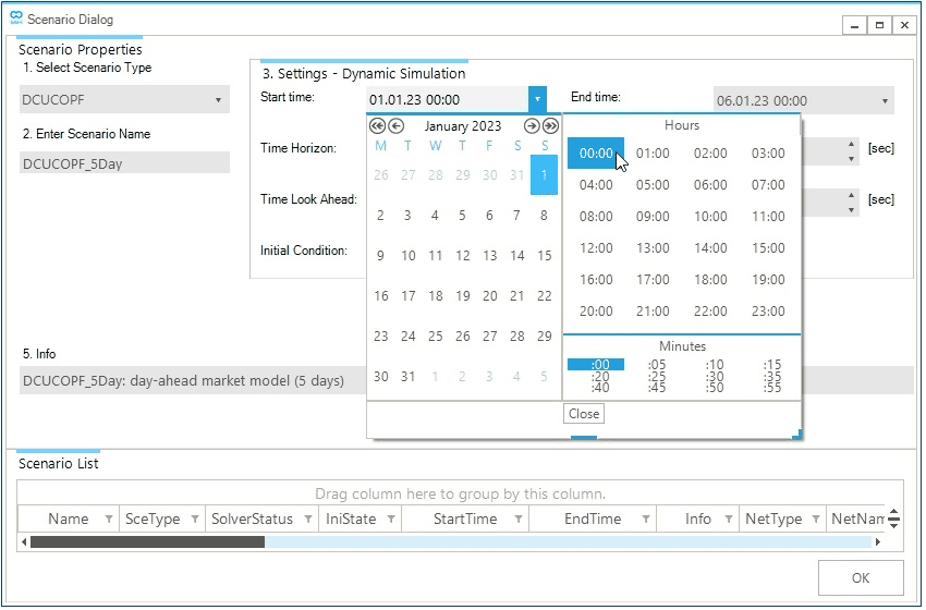
Firstly, you will start by defining the scenario TimeWindow, the difference between the scenario end and start times. Define the scenario StartTime as 01/01/2022 00:00 by navigating to the drop-down menu, as shown in Figure 1. Now, define the scenario EndTime by typing 06/01/2022 00:00 in the corresponding text box. This time definition means your scenario TimeWindow is of five days or 120 hours.

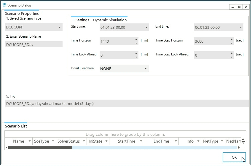
Secondly, you will define the duration and time step of each optimization. The time horizon describes a fraction of the time window used for each consecutive optimization; in this case, you will define a daily optimization with five consecutive optimizations. Enter a TimeHorizon of 1440 minutes (number of minutes in a day: 24 hours/day multiplied by 60 minutes/hour). The time step describes a fraction of the time window to discretize the scenario into distinct points in time to calculate the system’s variables. As previously stated, you will use an hourly resolution. Enter a TimeStep of 3600 seconds (number of seconds in an hour: 60 minutes/hour multiplied by 60 seconds/minutes).

2.2. Optional settings

Finally, there are optional settings that you can define. This tutorial will provide an overview of how these properties affect the DCUCOPF scenario. In future tutorials, you will analyze their effects with different case studies.

The TimeLookAhead is an additional time that extends each consecutive optimization (TimeHorizon plus TimeLookAhead). Adding the look ahead increases the model accuracy by using the information within the look ahead to influence the decisions of the network state beyond the end of the optimization window. The look-ahead can be considered as forecasted data for the day-ahead market optimization.
The TimeStepLookAhead is similar to the TimeStep, it describes the discretized time intervals for the look ahead period. This value is either equal to or longer than the scenario time step.
The InitialCondition defines a SAInt state file (.econ) from a previously executed scenario associated with the same network to input an initial state to the optimization model.

3. Create the scenario file

The final section you will be using is the 5. Info Section, here you can add additional information about the scenario. Enter the following info DCUCOPF_5Day: day-ahead market model (5 days), as shown in Figure 2. Once completed, click on OK at the bottom of the window. A prompt will show up that indicates the scenario was created successfully. Close the window or press OK to continue.

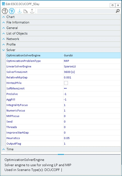
Figure 2. Scenario DCUCOPF_5Day settings defined.

4. Scenario solver setting

The DCUCOPF scenario in SAInt uses an external solver to evaluate the mathematical optimization problem. You have the possibility of changing and customizing the settings of the external solver via the scenario editor. Open the scenario editor by going to the scenario tab and pressing ESCE. You can change all the scenario properties in this editor window, but you will focus on the solver section as shown in Figure 3. Ensue the SolverType is Gurobi, the SolverTimeLimit is set to 3600 [s] and RelativeMipGap is 0.001 [-]. The SolverType property defines which external solver will be used for the market optimization. Meanwhile, the SolverTimeLimit and RelativeMipGap allows the user to tune the duration and accuracy of the optimization.

For additional information on the solver and other scenario settings, read the DCUCOPF section in the reference guide.

Figure 3. Scenario solver settings in the scenario editor.