Step 3: Run a Combined Simulation Scenario

Thanks for enduring up to this point! You are finally ready to run the combined simulations.

You have created a hub system by coupling two existing single-energy carrier networks. You defined a "scenario" by merging two coherent and aligned scenarios from the contributing systems. You are aware of the peculiarities of the events associated with coupling objects and the role of the "control mode" in defining their properties in all contributing systems. In this step, you will explore the dynamic of the coupled system in four different simulations.

1. Run a steady state combined simulation

Please, make sure to have the steady state gas scenario STEADY.gsce and the electric steady state ACPF scenario Steady_ACPF.esce open. A quick way would be to check the active scenarios reported at the bottom of the main SAInt window. Alternatively, close any scenario you have active and load them again using File>Open Open Gas Network Scenario and File>Open Open Electric Network Scenario from the Scenario tab.

Open the events table for each scenario and uncheck (i.e., set to False) the property Active for the following events:

QSET equal 1 ksm³/h for GSUP.P2H2 in STEADY.gsce;
PSET equals to 8 MW for EDEM.CS1 in Steady_ACPF.

This action is not strictly necessary, but helps in remember on which system the control mode of the object is.

Run the combined simulation from the Simulation tab by selecting the option Execute Combined. SAInt will inform on successfully completing the combined steady state simulation. Have a look at the content of the log window. No error messages or warnings; that’s great!

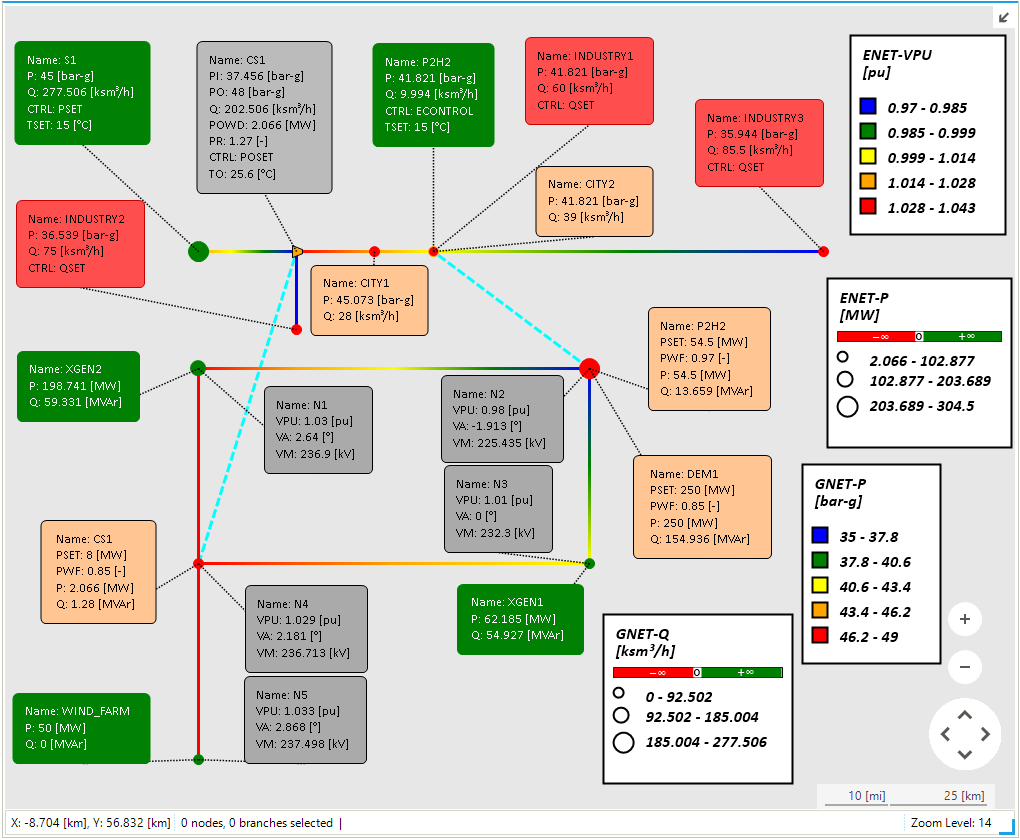
You can now compare the solution you got with Figure 1 where you have labelled all main facilities and externals. Note that the labels for the coupling objects report (in blue) the same values as in the labels for the single-energy carrier objects. This is obviously expected. Furthermore, note the type of control reported for the gas object GSUP.P2H2, it is ECONTROL. This shoes a good example of how coupling objects operate.

Before proceeding, remember to save your project.

Figure 1. Solution for the combined simulation for the gas steady state scenario STEADY.gsce and the electric steady state ACPF scenario Steady_ACPF.esce.

2. Run a dynamic combined simulation

You are switching to the combined dynamic simulations.

The first combined simulation you are going to explore requires the dynamic gas scenario BAU_DYNAMIC.gsce and the electric quasi-dynamic QuasiDynamic_ACPF.esce. Please, open those scenarios using the menu File Open in the Scenario tab or from the project explorer.

Quickly recheck that the scenarios are coherent and aligned by scrolling through their properties in the property editor. Look at the profiles to verify that the ones for gas are starting at 06:00 in the morning and the ones for electricity are starting at 00:00 in the morning. Finally, let’s control the events of the scenarios.

The gas scenario is good to go. You have only events for the demand externals, and the electric-drive compressor station inherits the control mode and set point from the initialization state. The electric scenario requires some minor tuning. You have to unselect (i.e., set to False) the property Active for the object EDEM.CS1. SAInt is going to ignore the event anyway, but the clarity of the scenario is improved in this way.

Run your first combined dynamic simulation from the Simulation tab by selecting the option Execute Combined. SAInt will inform on successfully completing the simulation. Take your time to go through the log in the log window. Though you don’t have errors or warnings, it is informative to look at it.

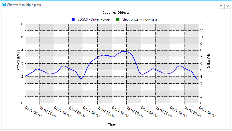
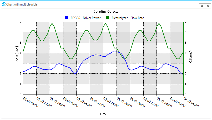
Plot the behavior of the coupling objects with the following command.

nplot('HUB.HUB_CS1.POWD;left;[6,0,6];blue;title=Coupling Objects;legend=EDGCS - Driver Power', 'HUB.HUB_P2H2.Q;right;[12,0,12];green;legend=Electrolyzer - Flow Rate')

You can see in Figure 2 how the demand for electricity in the compressor station changes during the simulation, and the flow rate of newly produced hydrogen at the electrolyzer.

Figure 2. Driver power of the electric-driven gas compressor station EDGCS.HUB_CS1 and flow rate of the synthesized hydrogen at the electrolyzer P2G.HUB_P2H2 in the combined simulation of the dynamic scenarios BAU_DYNAMIC.gsce and QuasiDynamic_ACPF.esce.

The nplot command explicitly uses objects of type HUB to stress how objects are coupling entities. Alternatively, you could have used EDGCS.HUB_CS1 and P2G.HUB_P2H2.

Save your project and close the opened scenarios.

In our second combined simulation we are going to check the impact of "issues" at the supply point S2. Load the dynamic gas scenario S1_DYNAMIC.gsce and the electric quasi-dynamic QuasiDynamic_ACPF.esce. Please, open those scenarios using the menu File Open in the Scenario tab or from the project explorer.

As before, check in a sequence that the following conditions hold, and change properties if necessary:

the contributing scenarios must be coherent and aligned;
the scenario profiles must match your modeling needs;
the events for the coupling objects must be adequately defined for the system holding the control mode. All unnecessary events on the other contributing system should be removed or inactive.

Similarly to the first combined simulation, the contributing gas scenario does not need any change, while in the electric scenario the event related to EDEM.CS1 has to be inactive.

Run your second combined dynamic simulation from the Simulation tab by selecting the option Execute Combined. SAInt will inform on completing the simulation. Take your time to go through the log in the log window. There is no error, but, as expected, you have some warnings concerning pressure issues at N3 for the industrial external GDEM.INDUSTRY2.

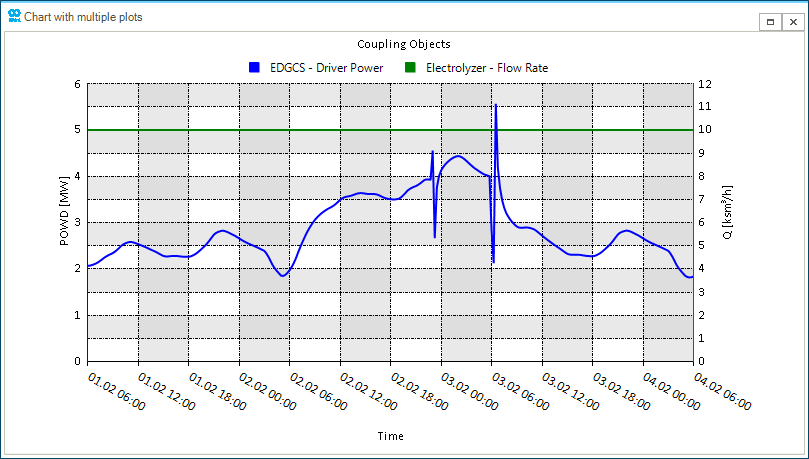
Plot the behavior of the coupling objects with the following command.

nplot('HUB.HUB_CS1.POWD;left;[6,0,6];blue;title=Coupling Objects;legend=EDGCS - Driver Power','HUB.HUB_P2H2.Q;right;[12,0,12];green;legend=Electrolyzer - Flow Rate')

You can see in Figure 3 how the demand for electricity of the compressor station changes during the time window of the contingency on the supply point GSUP.S1 (i.e., between 23:00 on 02/02/2020 and 06:00 on 03/02/2020). You see some transients (i.e., spikes) that you could be asked to manage. The electrolyzer is untouched by such events.

Figure 3. Driver power of the electric-driven gas compressor station EDGCS.HUB_CS1 and flow rate of the synthesized hydrogen at the electrolyzer P2G.HUB_P2H2 in the combined simulation of the dynamic scenarios S1_DYNAMIC.gsce and QuasiDynamic_ACPF.esce.

Save you project and close the opened scenarios.

The third and last combined simulation combines the dynamic gas scenario H2_DYNAMIC.gsce and the electric quasi-dynamic QuasiDynamic_ACPF.esce. Please, open those scenarios using the menu File Open in the Scenario tab or from the project explorer.

Again, verify the following:

the contributing scenarios are coherent and aligned;
the scenario profiles match the modeling needs;
the events for the coupling objects are correctly defined for the system holding the control mode. All unnecessary events on the other contributing system should be removed or inactive.

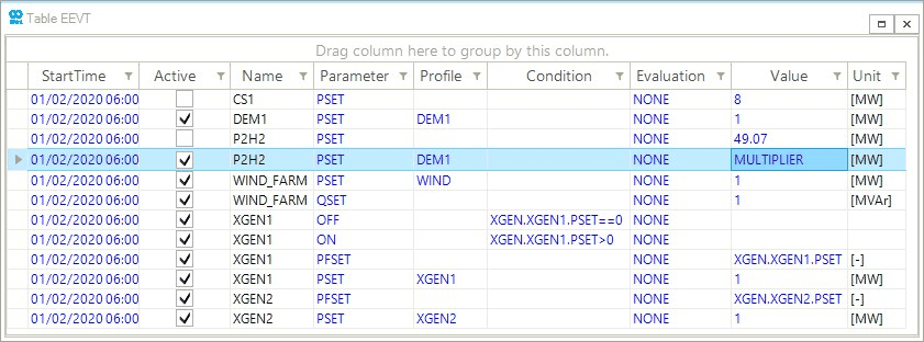
Uncheck any event, except the one for temperature, related to GSUP.P2H2 in H2_DYNAMIC.gsce. Modify the electric scenario as follow:

de-activate the events linked to EDEM.CS1;
de-active the event PSET for EDEM.P2H2;
in the command window, type MULTIPLIER=0.15, and then add a new event PSET to EDEM.P2H2 and in the Value field, write MULTIPLIER;
specify DEM1 in the field PROFILE for the previous newly created event.

The revised version of the events table should look like Figure 4. Here, you have showcased a new feature of SAINt: you can define constants and use them in expressions to adjust the value of a property. Why do you introduce this constant? The answer is simple you do not want to introduce a new profile for the electricity demand of the electrolyzer. So you repurpose the existing profile DEM1 to fit your needs!

Figure 4. Revised events table for the electric scenario QuasiDynamic_ACPF.esce.

Constants defined in the command window are temporary and are not saved with your project. Remember to generate them again!

Run the combined dynamic simulation from the Simulation tab by selecting the option Execute Combined. SAInt will inform on completing the simulation. Take your time to go through the log in the log window. Great! No errors or warnings.

Finally, plot the behavior of the coupling objects with the following command.

nplot('HUB.HUB_CS1.POWD;left;[7,0,7];blue;title=Coupling Objects;legend=EDGCS - Driver Power','HUB.HUB_P2H2.Q;right;[7,0,7];green;legend=Electrolyzer - Flow Rate')

You can see in Figure 5 how the flow rate changes during the simulations, while the electric-driven compressor station is not affected.

Figure 5. Driver power of the electric-driven gas compressor station EDGCS.HUB_CS1 and flow rate of the synthesized hydrogen at the electrolyzer P2G.HUB_P2H2 in the combined simulation of the dynamic scenarios H2_DYNAMIC.gsce and the revised QuasiDynamic_ACPF.esce.

Save your project and close the opened scenarios.