Step 1: Create an Electric Network Model
Start the tutorial by creating an electric model used to carry out a QuasiDynamic simulation over seven days. The electric model is comprised of four lines, two fuel generators, one fuel object, two generic generators, one wind generator, one solar generator, one demand, and two storage objects. The model considers a look ahead period of 1 day.
1. Create a new project and build your network
You have learned the basics of drawing your network in the beginner tutorials. Now it is time to put into good practice your knowledge. The main advantage of building your system directly in the GUI is that you take the time to define all relevant details of the nodes, the branches, and the externals. Furthermore, topological consistency is immediately enforced. For simple projects, this approach is fantastic!
For more complex networks, manually drawing can be time-consuming. A better strategy would be to use templates in Excel™ or shapefile format to quickly organize your data and then take advantage of SAInt’s import capabilities.
1.1. Create a new project
The first thing you need to do is to create a new empty project and select the basic properties of your model. The project stores your new model and organizes data, scenarios, results, and simulation scripts. The project settings will address some fundamental aspects like units of measure, reference conditions, or type of equation used for friction or compressibility.
When launching the GUI, you see the default "New Project" space.
Click on  and select Save Project.
Please create a new folder named Tutorial-DCUCOPF-3 and select it.
The project is renamed out of the folder and saved there.
and select Save Project.
Please create a new folder named Tutorial-DCUCOPF-3 and select it.
The project is renamed out of the folder and saved there.
Now, select again and go to Settings.
In the new window, select "Units" tab and specify the set of units of measure and the currency you prefer.
In the tutorial, you will use commonly applied units from the International System and the euro as currency.
Remember to click on Apply!
1.2. Draw the tutorial network
Now that the project is ready, it is time to start creating your network. Go to the Network tab and select . Create a new directory named eNetwork1 inside the project folder and click Select Folder. A new simple network is generated.
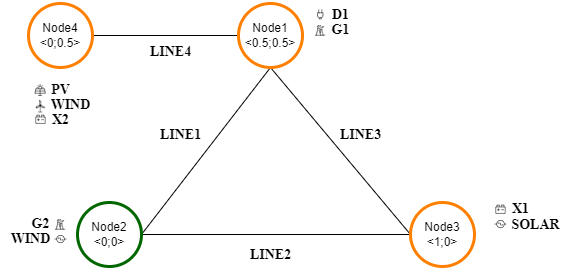
Use the information provided in Figure 1 to draw the tutorial network.
Start by changing the name of the two nodes: ENO_0 should be Node1, and ENO_2 should be Node2.
Select node Node1 now and, from the property editor, adjust its X-Coordinate (property X) to 0.5 km, and Y-Coordinate (Y) to 0.5 km.
Continue by adding the new nodes and lines.
Complete the system’s geometry and topology by updating the nodes' names.
Once the network is complete, it is time to add the externals. Follow the scheme in Figure 1 and add to each node the corresponding external with the correct name.
|
In Figure 1 under the node name, the location is expressed with coordinates in kilometers (e.g., node Node1 is at x 0.5 km and y 0.5 km). The node color follows SAInt convention: green for supply, red for demand, orange for mixed, and light grey for nodes without externals. |
1.3. Edit objects properties
Use "tables" to quickly edit the objects' properties you have just created.
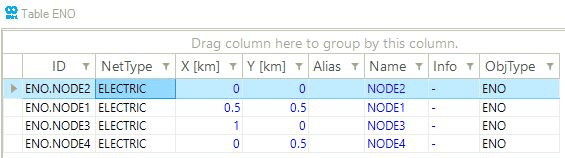
For example, from the Table tab of the GUI select  to open the table of nodes of the model.
You can arrange or hide the existing columns and show new columns with the option "Show Column Chooser" by right-clicking in the blank space below the table ("Drag column here..").
Figure 2 shows an example of the possible layout of the table.
Edit the properties of the nodes using the data provided in Table 1.
Leave the default value for all other properties not mentioned in the table.
to open the table of nodes of the model.
You can arrange or hide the existing columns and show new columns with the option "Show Column Chooser" by right-clicking in the blank space below the table ("Drag column here..").
Figure 2 shows an example of the possible layout of the table.
Edit the properties of the nodes using the data provided in Table 1.
Leave the default value for all other properties not mentioned in the table.
Click here to view the properties of the nodes of the tutorial network.
| Name | X-Coordinate | Y-Coordinate |
|---|---|---|
|
|
|
NODE2 |
0 |
0 |
NODE1 |
0.5 |
0.5 |
NODE3 |
1 |
0 |
NODE4 |
0 |
0.5 |
Follow the same approach for the electric lines. Start by opening the table for that object type, then adjust its columns and edit the properties. Use the data provided in Table 2 for electric lines.
Click here to view the properties of the electric lines of the tutorial network.
| Name | FromNodeName | ToNodeName | DefReactance | DefMaxActivePower |
|---|---|---|---|---|
|
|
|
|
|
LINE1 |
NODE1 |
NODE2 |
0.01 |
50 |
LINE3 |
NODE1 |
NODE3 |
0.01 |
150 |
LINE2 |
NODE2 |
NODE3 |
0.01 |
150 |
LINE4 |
NODE4 |
NODE1 |
0.01 |
200 |
Once the network topology has been created, populate the nodes with the external objects.
Create the demand and the four renewables generators.
In SAInt, solar (and wind) generators can be created as either XGEN or as PV generators (or WIND).
If solar is modeled as PV object, historical weather resource data can be downloaded from external data providers as explained in integrating weather resource data.
Select NSRDB-PSM3 as the Select Provider, 2010 for the Year and 30 minutes for the Interval.
In this tutorial, you are going to create two solar and two wind generators, respectively, as XGEN and PV / WIND objects.
The modeling differences in SAInt for a solar generator are visible in Table 3 and Table 4.
Click here to view the properties of the solar modeled as an XGEN external object.
| Name | NodeName | DefMaxActivePower |
|---|---|---|
|
|
|
SOLAR |
NODE3 |
100 |
Click here to view the properties of the solar modeled as a PV external object.
| Name | NodeName | DCACRatio | Tilt | Latitude | Longitude | ArrayType | ModuleType | DefMaxActivePower |
|---|---|---|---|---|---|---|---|---|
|
|
|
'Tilt` |
|
|
|
|
|
PV |
NODE4 |
1.2 |
25 |
25.74 |
-80.27 |
OneAxisTracker |
Premium |
100 |
The modeling differences in SAInt for a wind generator are visible in Table 5 and Table 6.
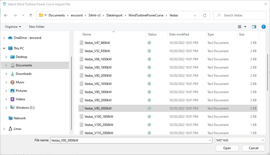
The wind turbine power curve used for the WIND object named WINDFARM is the VESTAS_V90_3000KW.
Before applying the wind turbine power curve to the WIND object is necessary to import from as shown in Figure 3.
An exhaustive list of wind turbine power curves is available at C:\...\DataImport\WindTurbinePowerCurve.
Once successfully imported, access the property extension WTPCName and, using ▼ select the wind turbine power curve.
Click here to view the properties of the wind modeled as an XGEN external object.
| Name | NodeName | DefMaxActivePower |
|---|---|---|
|
|
|
WIND |
NODE2 |
150 |
Click here to view the properties of the wind modeled as a WIND external object.
| Name | NodeName | HubHeight | Latitude | Longitude | DefMaxActivePower |
|---|---|---|---|---|---|
|
|
|
|
|
|
WINDFARM |
NODE4 |
160 |
25.74 |
-80.27 |
80 |
The last two generators in the network are fuel generators with two different fuel objects.
The fuel generator properties are split among Table 7 and Table 8.
Finally, the fuel objects GAS and COAL cost 0.1 €/MMBTU and 2 €/MMBTU (property = FuelPriceDef).
Click here to view the fuel generators' properties (part 1) modeled as an FGEN external object.
| Name | NodeName | FuelName | LinFuelConsCoeff | DefMaxActivePower |
|---|---|---|---|---|
|
|
|
|
|
G1 |
NODE1 |
COAL |
10 |
350 |
G2 |
NODE2 |
GAS |
8 |
150 |
Click here to view the fuel generators' properties (part 2) modeled as an FGEN external object.
| Name | DefMinActivePower | DefVOMPrice | DefStartUpPrice |
|---|---|---|---|
|
|
|
|
G1 |
100 |
3 |
3000 |
G2 |
20 |
2 |
1500 |
You are almost there! The last two objects of this network are the storage objects that are described in Table 9 and Table 10.
Click here to view the electric storage properties (part 1) modeled as an ESTR external object.
| Name | NodeName | DefMaxStorageCapacity | ChargeEfficiency | DischargeEfficiency |
|---|---|---|---|---|
|
|
|
|
|
X1 |
NODE3 |
90000 |
0.82 |
0.82 |
X2 |
NODE4 |
90000 |
0.82 |
0.82 |
Click here to view the electric storage properties (part 2) modeled as an ESTR external object.
| Name | DefMaxChargePower | DefMaxDischargePower |
|---|---|---|
|
|
|
X1 |
5 |
5 |
X2 |
5 |
5 |
|
Remember to save your network and your project from time to time. |
1.4. Use a template
Indeed, the major advantage of creating your network directly in SAInt is that you have complete control of all steps. You can double-check objects' properties and network’s details. And you can customize your project right away. But this scales up with the size of your network! And when you go big, you may be looking for alternatives to create your model and transfer the data.
SAInt allows for importing networks and data in alternative ways. You can use Excel templates to easily collect and organize data from multiple sources in a simple table layout.
Look at the files in C:\...\Documents\encoord\SAInt-v3\DataImport to find the templates.
Check the section data exchange for an in-depth description of the templates' structure, mandatory fields, data organization, and procedures for importing.
For this tutorial, you can use an Excel template.
Use the Excel template "ENET-beginner-tutorial-3.xlsx" available in the sub-folder .\Energy Markets\Tutorial 3 of the folder Tutorials in the directory (C:\Users\...\Documents\encoord\SAInt-v3\Projects).
Save it in your project directory and select from the Network tab.
The import procedure will ask for the Excel template and the name and location of the new network.
A message will inform you of the successful import, indicating the number of nodes and branches imported.
The new network is available in the active project, and you are ready to go.
|
Try to create your own version of the template. Start with an empty one and use the previous section’s nodes, branches, and external’s details to fill the template in. This procedure is an excellent exercise for understanding how templates work. |