Step 7: Create Time Profiles for Events in a Quasi-Dynamic Scenario

Quasi-dynamic or time-dependent variables in SAInt are modeled using time profiles in the scenario. Each profile comprises equidistant data points describing an object’s property change over time. This step will focus on developing profiles to define the demand points of your system in the SAInt GUI. The objective is to understand how different properties affect a profile and learn how to visualize, create, and edit profile data points.

By adding profiles to the events of your scenario, you are ready to complete a quasi-dynamic simulation.

1. Open the profile table

In this quasi-dynamic simulation, the demand HDEM.HDEMAND5 will use an absolute profile, which is, in this case, a time series of hourly values, while all other demands will be modeled with standardized, average fixed profiles.

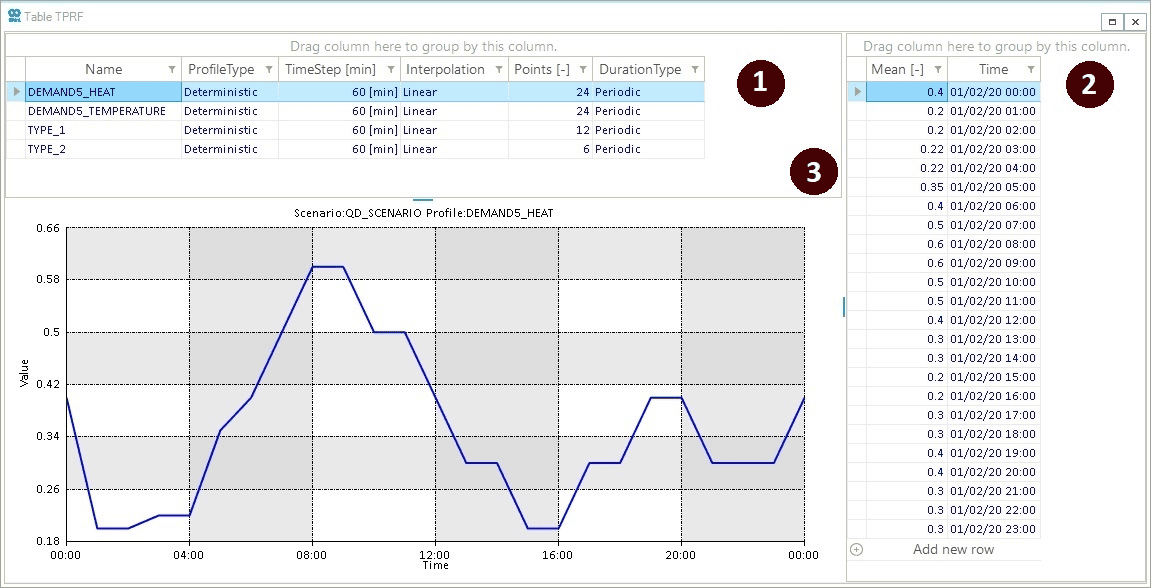
Let’s start by opening the profile table by going to the scenario tab and selecting TPRF. The profile table is divided into three main sections, as shown in Figure 1:

Profile description table (❶): this section allows the user to see and edit the properties of the profiles. You can edit the profile name, type, and time step. Additionally, you can directly create and delete profiles for the scenario file.
Profile data table (❷): this section displays the time series data points of the currently selected profile (highlighted in light blue in the profile description table). Here, you can directly edit the profile by changing, adding, or removing any cell of the profile data series. The column Mean must be filled to define the profile’s data points. Here the term "Mean" does not imply the concept of average because you are using deterministic profiles. So, it is just a name for the column. The column Time indicates the exact time of each step in the profile based on the starting time of the scenario. By default, SAINt displays also a column named Deviation, which is only used in stochastic profiles, and which is hidden in Figure 1.
Profile chart window (❸): this section plots the values of the profile data points against the scenario time window to visualize the dynamic behavior of the currently selected profile.

Figure 1. Profile for the heat demand component of the object HDEM.HDEMAND5 in the profile table. The three sections of the profiles table are shown with the symbols ❶, ❷, and ❸.

2. Create a profile

We will now create the profile shown in Figure 1. Go to the profile description table, right-click in any empty spot and select Create Profile. A new profile will appear, and you can now edit the profile properties. You will use the default properties for all your profiles but edit the profile’s name. So, for your first profile, change the value in the Name column to DEMAND5_HEAT.

2.1. Enter and visualize profile data

By default, you will notice that when a new profile is created, you have only two data points set to a value of 1. Now, you can edit the profile data points in the profile data table (❷ in Figure 1). Under the column Mean, enter the corresponding data points for the DEMAND5_HEAT provided in Table 1.

You can edit profile data points manually by selecting the desired cell, then overwriting the value and pressing Enter to save the new value in the cell. Press Down to select the following row and repeat the process. However, once you add new data points to the profile data series by pressing Enter, you will automatically jump to the following cell.

You can repeat these few steps and create the profiles named DEMAND5_TEMPERATURE, TYPE_1 and TYPE_2.

Finally, it is time to clarify two important points:

The profile length can be different from the simulation time window. This is the case of TYPE_2 where you have only six points. SAInt allows for periodically repeating the profile if it is shorter than the simulation length. But other options are available too.
When using an absolute profile, like for DEMAND5_TEMPERATURE or DEMAND5_HEAT, remember to set the value of the associated event to 1 and choose the correct unit of measure (e.g., °C). SAInt will compute the demand at 01:00 a.m. by multiplying one by the value in the profile (i.e., 1 x 20). The profile defines the absolute magnitude of the final value. When using standardized, average fixed profiles, the event value determines the absolute magnitude, while the profile is the relative weight. For TYPE_1 at 05:00 a.m. you may have an absolute event value of 0.5 MW to be multiplied by 0.90 (i.e., a relative decrease of 10 %), equal to 0.45 MW.

Click here to view the profile data.

Table 1. Values for the profiles in the quasi-dynamic simulation.
DEMAND5_HEAT	DEMAND5_TEMPERATURE	TYPE_1	TYPE_2
Mean	Mean	Mean	Mean
0.4	30	0.8	0.95
0.2	20	0.8	0.95
0.2	20	0.9	1
0.22	24	0.9	1.1
0.22	24	0.9	1.1
0.35	28	0.9	1.1
0.4	30	1
0.5	32	1.1
0.6	32	1.1
0.6	32	1.1
0.5	31	1.1
0.5	31	1
0.4	30
0.3	26
0.3	26
0.2	20
0.2	20
0.3	26
0.3	26
0.4	30
0.4	30
0.3	26
0.3	26
0.3	26

2.2. Include profile data

When you have many profiles or some of them are long, the manual editing approach is cumbersome. For this situation, SAInt allows using an "include" feature to input profiles from an existing profile file (*.prfl). Before continuing with the following steps, ensure you have a copy of the file "Profile_data.prfl" from the tutorial directory. Right-click the blank space in the profile description table and select Include Profile(s). This will open a window asking which profile file to open. Locate the profile file from the zip folder and press Open. A prompt that the profiles have been successfully loaded should appear. Press OK or close the window to continue.

The newly included profiles' names may be changed to avoid any conflict with the existing ones. This situation will be your case because you have already created all three profiles. So an "_1" is appended to the included profiles.

If you have duplicated profiles, remove them by selecting one at a time and right-click on its row to access Delete Profile(s).

Alternatively, you can include profiles by using Include > Profile(s) To Thermal Scenario (TSCE) from the "Scenario" tab.

Or, you may import profiles by using Excel templates and Import > Profile(s) To Thermal Scenario (TSCE) from the "Scenario" tab.

3. Assign profiles to events

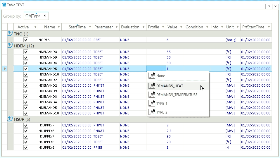
Move back or reopen the event table. You can select the tab "Map1: TNET" from the map window or the scenario tab by clicking on TEVT. Now you can associate events with profiles. Hoover the cursor over an empty column Profile cell and right-click. From the context menu, select the appropriate profile for the event, like in Figure 2. Proceed to match all events with the associated demand profiles.

Assign profiles in the following way:

DEMAND5_HEAT: to demand HDEMAND5 and event PHISET;
DEMAND5_TEMPERATURE: to demand HDEMAND5 and event TDSET;
TYPE_1: to events PHISET for demands HDEMAND2, HDEMAND3, and HDEMAND10;
TYPE_2: to events PHISET for demands HDEMAND4 and HDEMAND9.

Figure 2. Assign profiles to events in the event table of the scenario.

4. Save scenario profiles

To save your work, you will need to save the scenario file. Go to the scenario tab and select Save Save Thermal Network Scenario. This procedure will update the scenario file with the new profile data. Notice that the log window on the bottom right will inform you once the scenario has been saved.

Now, you are ready to run your quasi-dynamic simulation.