Step 2: Define Time-series Input Data

CEM scenarios typically require the following time-series information: forecast demand values for electric demand, availability profile of PV, and availability profile of wind. In this example, we will use hourly demand forecast, and historical availability profiles of PV and wind objects in the scenario.

For CEM scenarios, the majority of time-series information is contained in the file RepPeriodsTimeSeriesInput.csv. This file can be found in the Input folder of the tutorial material.

1. Defining the Demand Profile Data

We will use hourly timesteps to capture the operational details of this model. Therefore, we need a demand profile with 1 hour resolution. For one year, this translates to 8760 unique timesteps. Open the RepPeriodsTimeSeriesInput.csv in Microsoft Excel and see how this data has been entered in the column EDEM.LOCAL_DEMAND. Notice that these are normalized values. We will soon learn how to specify the actual demand peak using another input property.

2. Defining PV and Wind Availability Data

Similar to the demand profile, the availability of renewable generators for each hour is an important input for CEM. In the RepPeriodsTimeSeriesInput.csv file, these data are included under the columns PV.UTILITY_SCALE_PV and WIND.LAND_BASED_WIND, respectively. Since these are availability profiles, the values are normalized. The actual hourly generation of these units will depend on the optimal capacities decided by the solver.

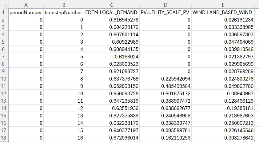
The screenshot below shows how the time-series data is entered in the CSV input file:

Figure 1. Time-series data input for CEM.

3. Representative Periods and Mapping to Timesteps

In this specific example, we use time-series data with 8760 unique timesteps to capture the profiles. Notice how the timestepNumber column in the RepPeriodsTimeSeriesInput.csv file starts at 0 and ends at 8759 (as seen in Figure 1 above). This model only has a single period with 8760 timesteps. This can be verified by noting that the periodNumber column of the input file has only one number (0). For larger models, it might be computationally efficient to represent the year as a collection of repeated representative periods.

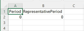
Regardless of having single or multiple periods, we need to specify how the time-series input data maps to operational timesteps. This is done using the PeriodToRepPeriodMapping.csv input file (as seen in the screenshot in Figure 2). Open this file in Microsoft Excel and see how the input data is entered. The input is trivial in this case since there is only a single representative period with 8760 timesteps. The data says that the period 0 maps to the representative period with ID 0. Since all the 8760 hours of the year are accounted for, there is no additional information needed here.

Figure 2. Mapping of representative periods.

A how-to will soon be available on usage of time domain reduction.