Step 3: Evaluate Data

This tutorial focuses on the IronPython scripting in the script editor of SAInt GUI. It explains the procedure for developing scripts using SAInt built-in functions to evaluate input properties and results. The IronPython scripting language can be used in SAInt GUI to automatize data analysis and processing tasks. Benefits of using IronPython’s notable features include:

Easy to develop user-defined functions.
High-level programming language and easy-to-read syntax.
Access to all network objects and properties.
Usage of built-in SAInt commands (e.g., plot, table, eval, etc.).
Usage of third-party modules.

1. IronPython script in the script editor

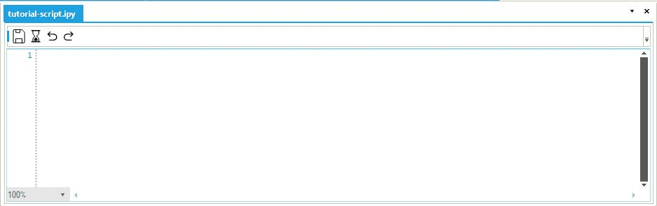
SAInt GUI has an integrated script editor which can be used to write and execute scripts. After execution, the results are displayed in the command window, the variables are saved in the workspace of SAInt GUI. To create a new IronPython script, click on Script Create New IronPython Script from the view tab. A new script editor appears as a tabbed document, as shown in Figure 1. Click on bt02 step03 02 to save the script to a user-defined location. To execute the script, click on bt02 step03 03 .

An existing IronPython script can also be loaded into SAInt GUI by clicking Script Open IronPython Script from the view tab.

Figure 1. New IronPython script editor.

2. SAInt built-in functions

SAInt has various built-in functions to be used in the script editor and command window. In the visualize data and analyze data tutorials, you learned how to use the plot and table functions in the command window. In this tutorial, you will use some of the other built-in functions in the script editor to evaluate different kinds of results.

Please refer to the evaluation functions section of the reference guide to learn more about the evaluation functions' syntax, input, and return expressions.

2.1. esum function

SAInt built-in evaluation functions (e.g., esum, emax, emean, ecount, etc.) are used to evaluate and aggregate input properties and results to understand the behavior of an object within a given time step or scenario time window. Use these functions to evaluate the total supply to the network, and the total demand of off-take DEMAND3 using the esum function for your simulation time window. Type the following commands in the script editor and execute:

esum('GSUP.SUPPLY1.Q.[ksm3/h].(%)'): Returns the total system supply equals to 19497.76 [ksm3] (rounded).
esum('GDEM.DEMAND1.Q.[ksm3/h].(%)'): Returns the total demand of the off-take DEMAND3 equals to 9760.0 [ksm3].

The "e" at the beginning of the function esum stands for "evaluate", and it is not related to an electric object.

2.2. emax and emin function

The emax and emin function can be used to evaluate the maximum and minimum value of an object parameter. You use the function emax to determine the peak hourly demand of an off-take point network (e.g., DEMAND3) and the function emin for the peak hourly demand at node NODE5. Type the following commands in the script editor and execute them:

emax('GNET.QMAX.[ksm3/h].(%)'): Returns the peak power demand of the network: 213.39 [ksm3/h] (rounded).
emin('GNO.NODE5.Q.[ksm3/h].(%)'): Returns peak hourly demand at the node NODE5 equals to -113.4 [ksm3/h].

A demand at a node is evaluated as an outflow and it has a negative value. This is why you need to use the emin instead of the emax function.

2.3. meantable function

In addition to the basic table function that you used in the analyze data tutorial, SAInt has other table functions to tabulate results and input properties. You will use the meantable function to evaluate the average hourly outflow of the demand objects over a 4[h] period. Use the following expression in the script editor and execute.

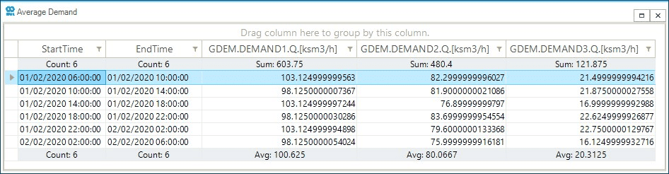
meantable('GDEM.DEMAND1.Q.[ksm3/h];title=Average Demand','GDEM.DEMAND2.Q.[ksm3/h]','GDEM.DEMAND3.Q.[ksm3/h]','4[h]','01/02/20 06:00','02/02/20 06:00')

As shown in Figure 2 the script returns a table where every row reports the average value of Q for each demand point over a four-hour time window.

Figure 2. Mean table for the four-hour average demand at each outflow point.

2.4. gmax and gmaxat functions

SAInt built-in graphical functions return graphical data to be used with the plot and table functions to plot and tabulate aggregated results and input properties. Use the gmaxat and gmax graphical functions with the table function to check which demand off-take point has the highest value at each time step during the time window 10:00 and 14:00 (10 a.m. and 2 p.m.) of the simulation.

You first need to make a small change to your event table, before diving into the example. Please, change the event GDEM.DEMAND1.QSET by setting the value to 80 ksm³/h, instead of 100 ksm³/h. After the change, run the simulation. Now you are ready to type the following command in the script editor and execute:

table(gmaxat('GDEM.%.Q.(%)'),gmax('GDEM.%.Q.(%)'),'01/02/2020 10:00','01/02/2020 16:00')

As observed in Figure 3 the table function returns the ObjectID of the particular demand point that has the highest outflow at every time step of the simulation in the time window between.

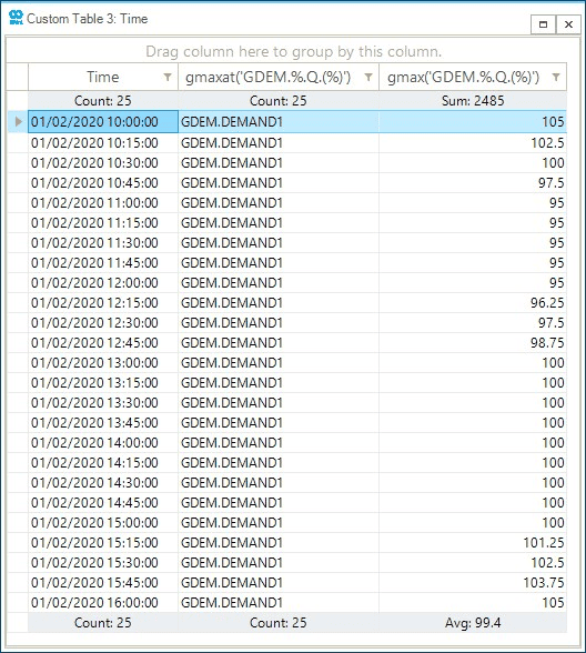
Figure 3. Table with ObjectID of the particular demand point that has the highest outflow at every time.

Please, remember to change back the value of GDEM.DEMAND1.QSET to 100 ksm³/h before closing your session.