Step 3: Create a Scenario and Run a Dynamic Simulation
Now that all pieces of the structure and topology of your model are in place, it is time to develop the scenarios and carry out the simulation. Your objectives are: to assess the impact of a possible contingency of the main supply point in the system GSUP.S1 and to check if changes in the hydrogen injection point GSUP.P2H2 may have effects on downstream users.
1. Create and run a steady state simulation
You begin by creating a steady state scenario and setting the initial state of your dynamic simulation. From the Scenario tab, select . Create a new steady state scenario named STEADY. Once the scenario is saved, open the scenario event table and add the events presented in Table 1 using either the map view or the model explorer.
| Object Name | Parameter | Value | Unit of Measure |
|---|---|---|---|
gNetwork1 |
|
5.0 |
°C |
gNetwork1 |
|
||
P2H2 |
|
15.0 |
°C |
P2H2 |
|
1.0 |
ksm3/h |
S1 |
|
15.0 |
°C |
S1 |
|
45.0 |
bar-g |
CITY1 |
|
28.0 |
ksm3/h |
CITY2 |
|
39.0 |
ksm3/h |
INDUSTRY1 |
|
60.0 |
ksm3/h |
INDUSTRY2 |
|
75.0 |
ksm3/h |
INDUSTRY3 |
|
85.5 |
ksm3/h |
PIPE4 |
|
0 |
°C |
CS1 |
|
48.0 |
bar-g |
Note that you have no event linked to the gas quality because quality tracking is active by default. You have also assigned a specific quality stream to the two supply points. So, you are covered.
|
If you want to disable quality tracking, add this extra event to gNetwork1 event |
The scenario is modeling the case where all supply points inject gas at a fixed temperature of 15 °C, and all branches experience an ambient temperature of 5 °C, except for PIPE4 for which the temperature is only 0 °C (this could be an aboveground pipeline).
When ready, launch the steady state simulation. You should get a solution like the one presented in Figure 1.
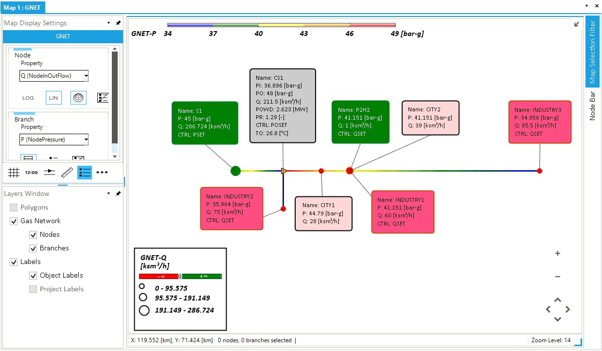
Note that you have set the legend for branches to describe the temperature in the pipelines. In this manner, you can visualize how the temperature changes in the system. For example, how it tends to stabilize in PIPE5 between INDUSTRY1 and INDUSTRY3. Or the impact of the compressor station, which increases the gas temperature to 26.8 °C. Or, you can see how the temperature drops along the aboveground pipeline PIPE4. Pressure-wise, the system has no problem, and all demands are fully satisfied.
1.1. Use a scenario template
This scenario is quite simple, and adding all events by hand is straightforward. But you could have used a scenario template as well. Scenario templates are handy in addressing more complicated events, with multiple options or values and conditions defined by external sources (e.g., co-simulation environments or SCADA systems).
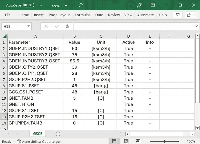
You can create your own template by looking at Figure 2 as an example. Check the section "scenario events template" for more details. Or you can use the one you have already prepared for you. Copy it from the Excel file "scenario-steady-state-events.xlsx" from the sub-folder .\Gas Networks\Intermediate Tutorial 1 of the folder Tutorials in the directory (C:\Users\...\Documents\encoord\SAInt-v3\Projects).
2. Create and run a dynamic simulation
You can now develop the business-as-usual dynamic scenario that you will use for implementing a contingency on the main supply point and some changes on the way you may use the electrolyzer for injecting hydrogen into the system.
As before, from the Scenario tab select . Create a new dynamic scenario named BAU_DYNAMIC (i.e., the business-as-usual dynamic). Set the scenario to start (StartTime) at 01/02/2020 06:00 (i.e., 6:00 a.m. on the first of February 2020). Set the scenario end time (EndTime) to 04/02/2020 06:00. The time step (TimeStep) is 600 seconds. Remember to select the scenario STEADY as the initial condition.
Once the scenario is created, you must define the profiles your external will follow during the simulation. You use a different deterministic profile for each external. Each profile covers three days with an hourly time step (i.e., 72 steps). The profile models a demand peak on February the 2nd. Its values are scaled so that the peak matches the event value. Interpolation between time steps is linear. Import the profiles using from the Scenario tab. Use the profile template provided with the Excel file "profiles.xlsx" available in the sub-folder .\Gas Networks\Intermediate Tutorial 1 of the folder Tutorials in the directory (C:\Users\...\Documents\encoord\SAInt-v3\Projects). Figure 3 shows an example of the profiles after the import.
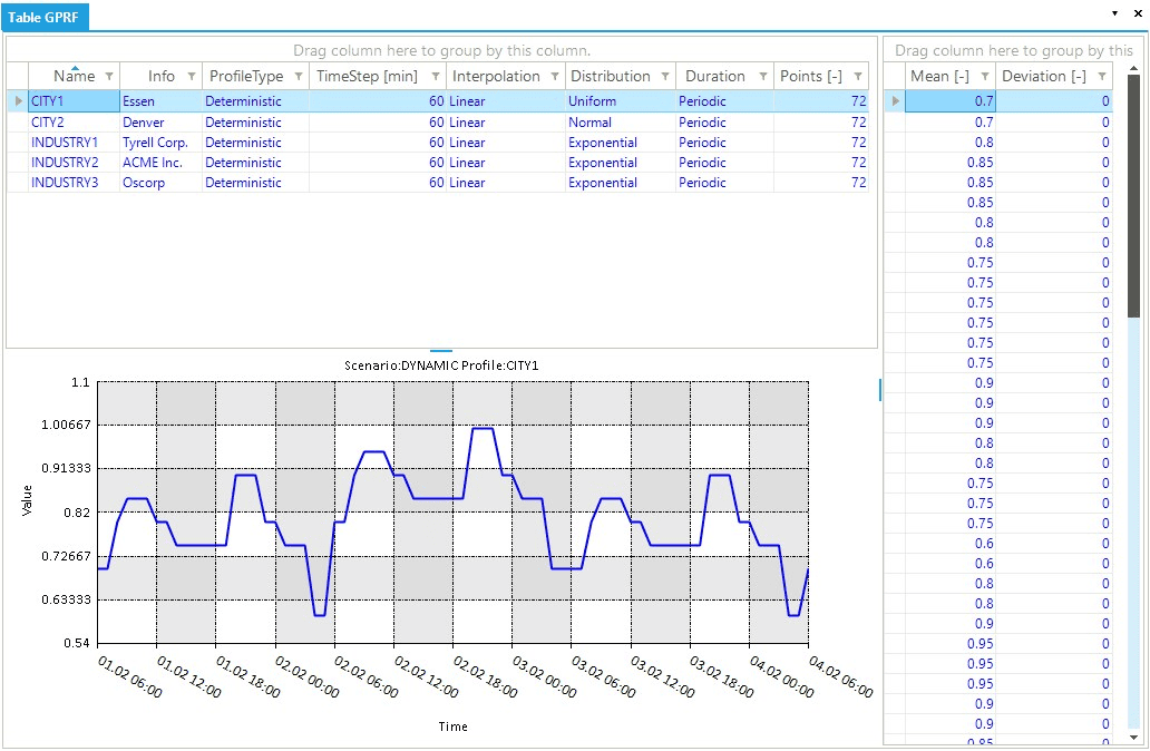
Distribution and Deviation are irrelevant for deterministic profiles. Duration can be set to any admissible value because the profile length matches the simulation length.Once the profiles are loaded, open the scenario event table and add the events presented in Table 2 using either the map view or the model explorer.
| Start Time | Object Name | Parameter | Profile | Condition | Evaluation | Value | Unit of Measure |
|---|---|---|---|---|---|---|---|
01/02/2020 06:00 |
gNetwork1 |
|
|||||
01/02/2020 06:00 |
CITY1 |
|
CITY1 |
NONE |
40.0 |
ksm3/h |
|
01/02/2020 06:00 |
CITY2 |
|
CITY2 |
NONE |
60.0 |
ksm3/h |
|
01/02/2020 06:00 |
INDUSTRY1 |
|
INDUSTRY1 |
NONE |
75.0 |
ksm3/h |
|
01/02/2020 06:00 |
INDUSTRY2 |
|
INDUSTRY2 |
NONE |
100.0 |
ksm3/h |
|
01/02/2020 06:00 |
INDUSTRY3 |
|
INDUSTRY3 |
NONE |
90.0 |
ksm3/h |
Finally, you can run the scenario and check the simulation log for possible problems. If everything goes as expected, there will be no error or warning. Congratulations!
Please, remember to save the project.
3. A contingency on the main supply point
You can simulate a possible contingency on the main supply point by creating new events altering the normal behavior of S1. Imagine you are this gas network’s transmission system operator (TSO). At S1, you have an agreement with the neighboring TSO for delivering at a minimum contractual pressure of 43 bar-g. In this period of the gas year, the overall demand is approaching the winter peak, so you have your gas delivered at higher pressure. But, at 23:00 (11 p.m.) of February the 2nd, your dispatching center observes a remarkable drop in pressure, down to 35.0 bar-g. After a few minutes, you receive a communication from the neighboring TSO informing the failure of one of their compressor stations. Repairs have started, but the normal values of the delivery pressure cannot be restored before 6:00 (6:00 a.m.) of February, the 3rd.
You can model this situation by using two new events, like the ones shown in Table 3, and check how your system reacts. First, select to copy the scenario BAU_DYNAMIC to a new scenario called S1_DYNAMIC. SAInt will create a copy of the scenario and switch to it. Now you can add the new contingency events.
| Start Time | Object Name | Parameter | Profile | Condition | Evaluation | Value | Unit of Measure |
|---|---|---|---|---|---|---|---|
02/02/2020 23:00 |
S1 |
|
35.0 |
bar-g |
|||
03/02/2020 06:00 |
S1 |
|
45.0 |
bar-g |
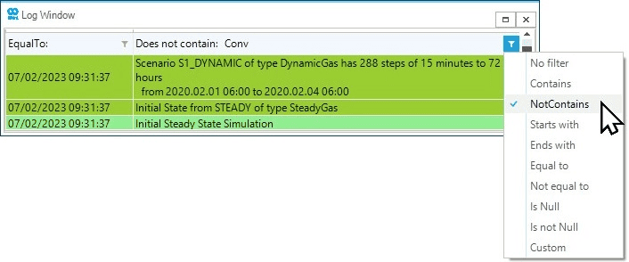
Let’s run the new scenario and check the log. You can use the filter function in the log window to extract all messages different from "Convergence step …". You can set up the filter by looking at Figure 4.
What you can read in the log is that:
-
You have problems at N3, where the pressure goes below the minimum pressure for the node. This problem affects the delivery to the external INDUSTRY2.
-
The compressor station hits its maximum pressure ratio value. Its control mode switches from
POSETtoPRMAX, reducing the flow. -
When S1 is restored at 45 bar-g, there is a transient where the flow at the supply point would be higher than the maximum allowed (
Qis higher thanQMAXfor S1). Similarly, the compressor stations' output pressure would spike above the value allowed by the maximum pressure ratio.
How would you manage the compressor station to cope with all these issues?
4. Changes in the way the electrolyzer is working
Assume that as the TSO, you are informed that the company operating the electrolyzer injecting hydrogen at the supply point P2H2 wants to increase its production from February the 1st at 13:00 (1 p.m.). Your contract with this company states that hydrogen injection can reach a maximum level that safeguards downstream network users from having hydrogen concentrations higher than 5 % in molar mass.
So the problem is to assess possible options of increased hydrogen supply satisfying the constraint on the downstream user INDUSTRY3.
Create a new scenario named H2_DYNAMIC by saving a copy of BAU_DYNAMIC and adding the event shown in Table 4.
| Start Time | Object Name | Parameter | Profile | Condition | Evaluation | Value | Unit of Measure |
|---|---|---|---|---|---|---|---|
01/02/2020 13:00 |
P2H2 |
|
9.0 |
ksm3/h |
Run the new scenario and check the concentration of hydrogen in the gas delivered to the industrial user downstream and the concentration at the injection point. Use the following plot command in the Command Window.
nplot('GNO.N7.NQ!X_H2;green;[6,0,12];title=Hydrogen concentration level for 9 ksm3/h;legend=User Point','GNO.N6.NQ!X_H2;blue;[6,0,12];legend=Injection Point','5[%-Mol];legend=Maximum concentration;red;dash;2')
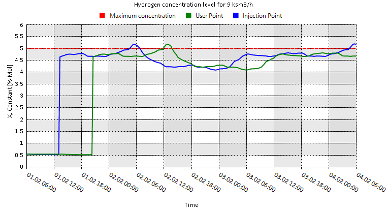
From Figure 5, you can conclude that an injection level of 9 ksm3/h is generally acceptable, but under peak hourly demand conditions, it could lead to unacceptable concentration levels for INDUSTRY3. Furthermore, at the end of the simulation, the model goes above the maximum threshold at the injection point. Finally, you can observe that hydrogen travels for around 7 hours before reaching the user in INDUSTRY3.
You could request the electrolyzer to inject at a maximum of 8.7 ksm3/h. Under this alternative, check the impact by plotting the results as before. Even during the peak, the concentration of hydrogen is safely below 5 %. Following, write in the Command Window:
inttable('GSUP.P2H2.Q.[ksm3/h]','72[h]').
The total amount of hydrogen injected during the simulation should be approximately 573.5 ksm3. Alternatively, you could better modulate the injection by dynamically checking the hydrogen concentration experienced by INDUSTRY3 at each time step.
Now deactivate the event QSET on S1 and add the new events shown in Table 5. You will use some conditions to modulate the use of the electrolyzer.
| Start Time | Object Name | Parameter | Profile | Condition | Evaluation | Value | Unit of Measure |
|---|---|---|---|---|---|---|---|
01/02/2020 13:00 |
P2H2 |
|
GDEM.INDUSTRY3.NQ!X_H2<=4.65 |
DoIFTRUE |
8.7 |
ksm3/h |
|
01/02/2020 13:00 |
P2H2 |
|
GDEM.INDUSTRY3.NQ!X_H2>4.65 |
DoIFTRUE |
7.0 |
ksm3/h |
Run the scenario and again check the concentration of hydrogen in the gas delivered to the industrial user downstream and the concentration at the injection point. Use the previous plot command in the Command Window, but remember to change the title.
By looking at the chart, you will see that you have been able to control the hydrogen concentration experience by the industrial user. The system reaches the maximum concentration around 12:45 on February the 2nd. But still, there is room for increasing electrolyzer usage. Check what is happening on February the 2nd, and consider that the total amount of hydrogen is 564.5 ksm3. Finally, there is a risky situation at the end of the simulation, where the concentration at the injection point is above 5 %.
Finally, try a different strategy. Instead of using a condition to change the injection level, define the actual value based on an expression where you calculate the flow as a percentage of the flow toward the industrial user. De-activate the current events associated with S1 and add a new one as presented in Table 6.
| Start Time | Object Name | Parameter | Profile | Condition | Evaluation | Value | Unit of Measure |
|---|---|---|---|---|---|---|---|
01/02/2020 13:00 |
P2H2 |
|
NONE |
|
ksm3/h |
As a final step, update Figure 5 and calculate the total amount of delivered hydrogen. You should see the system improvement regarding safe hydrogen levels from the chart. Furthermore, the total hydrogen supplied is around 618.7 ksm3 (i.e., approximately 8 % more than the 8.7 ksm3/h fixed flow!). But there is a possible catch! Try plotting the object’s outflow and control mode for P2H2. You will see that you have operated the facility at its maximum send-out capacity for a certain period. This condition could be an issue.
|
Look at the section list of table functions for more details on |