Step 5: Run the Steady State Simulation

You have done all the hard work and are ready to run your scenario assuming steady state conditions. Go to the simulation tab and press Thermal. During the scenario execution, you can track the progress by observing the status bar at the bottom of the screen. Additionally, the log window will display the simulation progress during each consecutive run. Once the simulation has finished, a prompt will appear with the message "Steady Thermal simulation completed successfully!". Close the window by pressing OK.

The log window is the first place to check when your simulation has problems or cannot be solved. SAInt keeps track of the status of the solver and informs the users of constraint violations, changes in the control mode of facilities, and, ultimately, failures. When no red lines are there, your simulation is successful. So, congratulations! Any condition preventing the simulation from finishing is summarized in the error message but must always be considered together with the actions taken by SAInt to deal with constraint violations (any yellow line in the log).

Light green lines inform the user on how the solver is progressing in solving the underlying mathematical problem and the convergence. Dark green lines describe the type of simulation, the model’s overall structure, the type of equation used to address the pipeline flow, or the reference conditions used for temperature and pressure. Also, the log reports default gas properties, the gas quality, and the status of temperature tracking.

SAInt always informs the user of the total computing time. So, you can manage your coffee breaks!

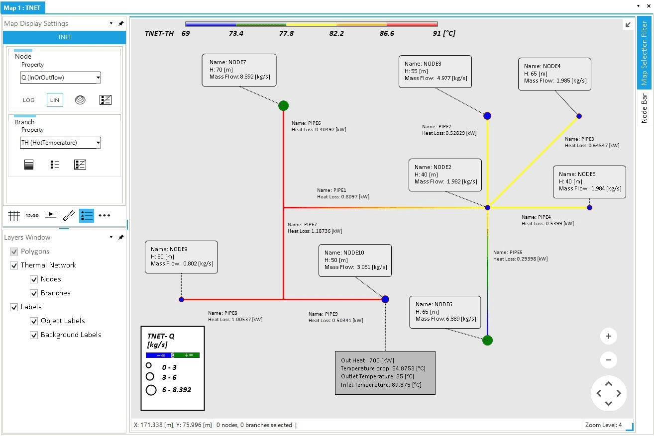
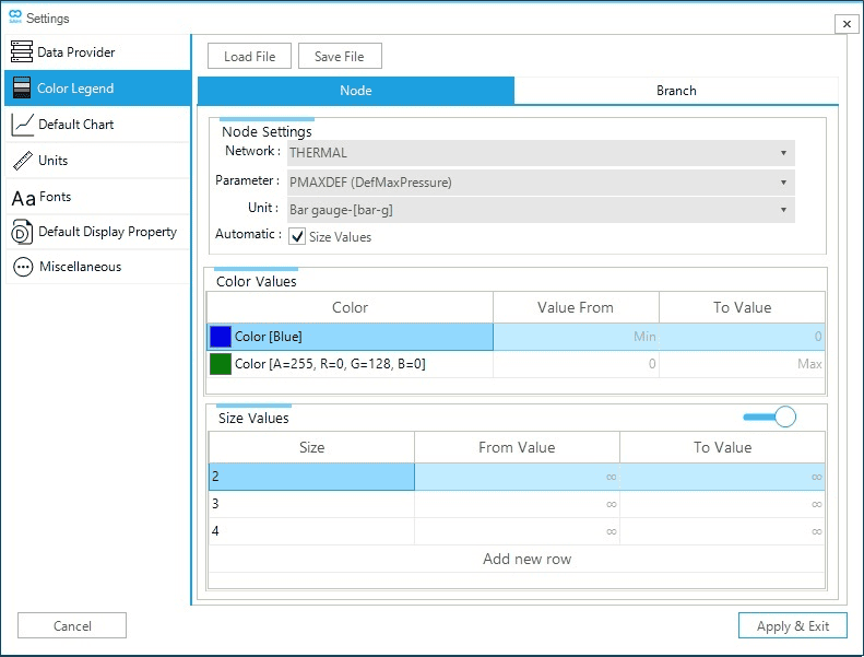
A quick way to explore the results of a steady state simulation is to check and assess the figures displayed with labels. For example, we can compare the different values of the mass flow across all nodes where external are present (Figure 1). We can support our assessment by using an ad hoc legend for the nodes to visualize better where we have the bigger flows. In the map display settings windows, under node, select the property Q (InOrOutflow). Click on the three dots icon ("Open Map Legend Settings" option) at the bottom right of the map display settings and go on the Node tab to personalize the size of the classes in the legend. Remember to turn to the right the sliding bar for the "Size Values", so that the classes are now editable. Untick the option for the automatic sizing of the nodes. Use three classes with "From value" of Min, 3, and 6. Any extra class can be removed from the context menu Delete Color Value(s) accessible from any cell. The final setup is shown in Figure 2.

You can also add new labels to demand externals to visualize details of each off-take point. For example, select HDEMAND10 and add a new label to the external. In the LabelInfo field type Out Heat : {@.PHI} Temperature drop: {@.TDROP} Outlet Temperature: {@.TO} Inlet Temperature: {@.TI}. Change the FillColor property to 187,187,187. See Figure 1 for an example of the outcome. You could add more labels to map all remaining externals and have graphical properties to help you distinguish between heat demands and heat supplies.

If we look at the results of the heat losses in the hot pipelines, we need to fine-tune the unit of measurement because megawatts are too big. Select all pipeline labels, right-click, and from the context menu, select Multi Edit. Open the label editor from the LabelInfo property. Change the line Heat Loss: {@.LOSS} to Heat Loss: {@.LOSS.[kW]}. Now, the value is reported using kilowatts (see Figure 1).

Finally, we can change the way pipelines are displayed. From the "Map Display Settings" under "Branch", select the property TH (HotTemperature). In this way we can color-code the pipelines based on the selected property (see Figure 1).