Run the SteadyACPF Simulation
In previous tutorial sections, we created all the elements needed to run the SteadyACPF simulation in SAInt. This step will focus on running the SteadyACPF simulation and visualizing relevant results using the object labels.
1. Execute the scenario
We have done all the hard work and are ready to run the power flow simulation. Go to the simulation tab and press Electric. During the scenario execution, the progress can be observed in the status bar at the bottom of the screen. Additionally, the log window will display the simulation progress during each consecutive run. Once the simulation has finished, a prompt will appear saying the simulation has been completed successfully. Close the window by pressing OK.
|
If the scenario execution fails for any reason, please review the previous steps and ensure everything was correctly defined. If the problem persists, please do not hesitate to contact our support team for guidance. |
2. Simulation logs in the log window
AC power flow simulation logs can provide useful information about the behavior of an electrical power system, including:
Total computation time: Provides the execution time needed to run the scenario file in seconds. Depending on your machine’s computational power, this scenario should take around 0.03 seconds.
Active Power Compensation Mode: It refers to a control strategy used to regulate the output of the generator to compensate for the active power losses in the system. In SAInt, two active power compensation modes can be defined:
-
PART: Generators participate in the compensation of active power unbalances proportionally to their participation factor
PFSET. In this scenario ,the default active power compensation mode PART is used. -
PRIOR : The generators with the highest PFSET are prioritized for the compensation of the active power unbalances. The active power compensation mode can be changed to PRIOR using the electric network scenario event from the model explorer (Figure 1).
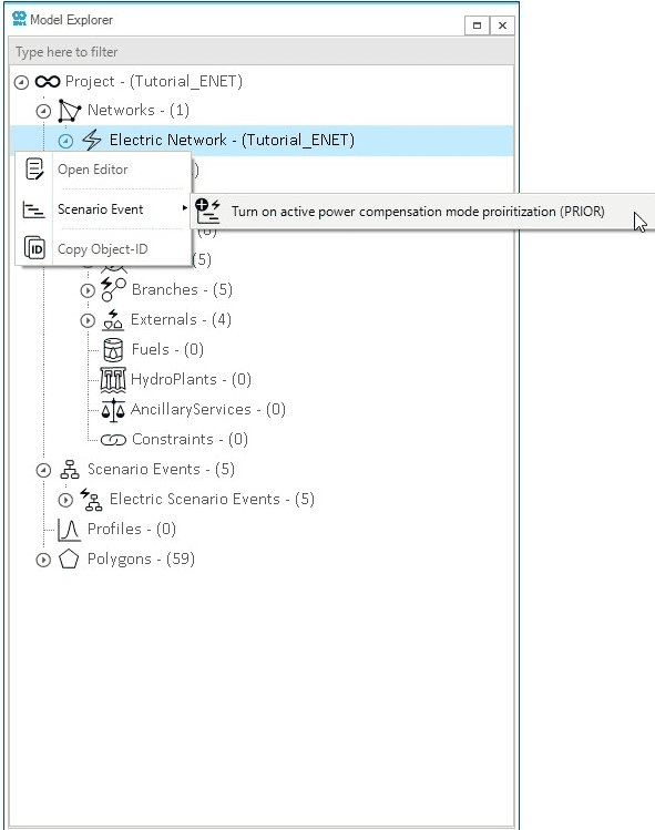
PRIOR.3. Analyze SteadyACPF results using object labels
The purpose of this simulation was to analyze the steady-state behavior of a flag-shaped power system, with the goal of verifying the correct operation of the system under normal conditions.
Inputs
-
One scheduled electrical demand.
-
Two voltage controlled generators with scheduled power supplies.
-
One wind farm with scheduled supply, and no voltage control (unit power factor).
-
Active power compensation distributed between two voltage controlled generators.
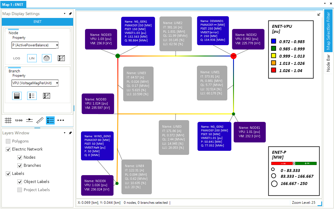
PART.The results of the Steady ACPF simulation displayed in Figure 2 show that the power system is operating normally under steady state conditions and the `PART`compensation mode.
-
Voltage magnitudes
-
The voltage magnitudes at all nodes were within the defined (
VMAXDEF) and (VMINDEF). Voltage at NODE1 and NODE3 is enforced by the generators NG_GEN2 and NG_GEN1, respectively.
-
-
Line loadings
-
The lines loading in terms of current (
LLI) is between [5.6%, 33.1%]. The lines loading in terms of apparent power (LLS) is between [10.6%, 62.6%].
-
-
Line Losses
-
The line losses (
PLandQL) are relatively small, indicating efficient power transfer between nodes.
-
-
Real and reactive power flows
-
The active power supply (
P) from the wind generator WIND_GEN3 is consistent with its scheduled supply (PSET), while the reactive power (Q) is 0 because of it’s unit power factor. -
The active power for generators NG_GEN1 and NG_GEN2 is higher than the scheduled supplies. The difference compensates the active power unbalance between scheduled supply and demand, due to losses in the electrical lines, while the reactive power flows are balanced.
-