Step 2: Analyze Data

Tables in SAInt can be used to analyze results concisely, especially with large amounts of data. Rather than showing trends and patterns with plots, SAInt shows the exact data values or derived statistics. Tables can be created both for a specific object type and combinations of object parameters to analyze and compare particular properties and results.

Moreover, the data can also be analyzed from the results tab of the property editor.

This tutorial analyzes some basic results using object tables and the property editor.

Tables in SAInt include several functionalities to filter, search, and add conditional formatting that can be customized using other features. A detailed explanation of all the features of object tables can be found here.

1. Object tables

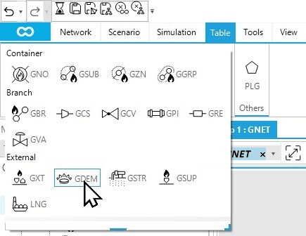
You will start by opening the table for gas demand points (GDEM) by clicking on the GDEM button from the table tab, as shown in Figure 1.

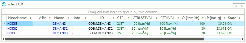
Figure 1. Access the table for demand points from the table tab.

The resulting GDEM table is shown in Figure 2. The table columns represent both the object’s control mode and output results. For example, the column with header CTRL and CTRLVAL indicate the obtained control mode for the object (i.e., QSET)` and the associated value for that control mode (i.e., a flow equal to 100 ksm³/h). Note that the result values in the table correspond to the display time of the map window. You can change the display time by using the time function in the command window. Compare the values in Figure 2, which are for the end of the simulation, with the ones obtained by entering the following expression time('02/02/2020 03:00') in the command window. The Q for DEMAND1 changes.

Figure 2. Table for the demand points.

1.1. Personalize table content

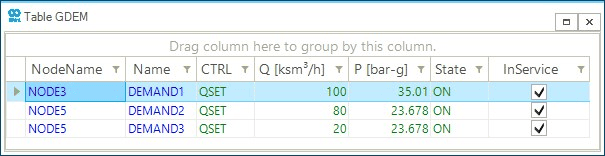
The object table’s columns are adjustable using the Choose Columns feature. Access the choose column dialog box by right-clicking on any of the column’s header rows and selecting Choose Columns option. In the dialog box, you will find the complete list of object properties that can be shown for that specific object type. To add a column, double-click on the desired property, and for unwanted columns, you can hide them by dragging and dropping them into the dialog box. You use the GDEM table to compare the following parameters: NodeName, Name, CTRL, Q [ksm3/h], P [bar-g], State, and InService as shown in Figure 3.

Figure 3. Demand points table with a personalized subset of columns.

SAInt object tables can be customized using other features. A detailed explanation of all the features of object tables can be found here.

2. Create customized tables

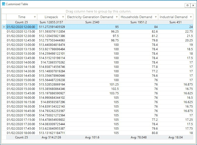
The object table can provide results for the given display time. On the other hand, the table function returns a user-defined expression(s) of object parameters over a specific time window. By default, the time window is based on the chart time window, like the plot function. You can use the table function to evaluate and compare the evolution and properties of objects in the simulation. For example, you can relate the total system linepack and the outflow at the demand off-take points. Use the following expression in the command window to create the custom table, as shown in Figure 4.

table('GNET.LP.[ksm3];header=Linepack,title=Customized Table','GDEM.DEMAND1.Q.[ksm3/h];header=Electricity Generation Demand', 'GDEM.DEMAND2.Q.[ksm3/h];header=Households Demand', 'GDEM.DEMAND3.Q.[ksm3/h];header=Industrial Demand', '01/02/20 12:00','01/02/20 18:00')

Figure 4. Example of a customized table in SAInt.

Please refer to the tables functions section of the reference guide to learn more about the table functions' syntax, input expressions, and specifications.

2.1. Add and edit summary row

Tables can also include a summary row(s) to quickly evaluate and compare summary results between different object parameters, including values such as count, average, sum, max, and min. You can add a summary row by right-clicking on the table’s top right corner and selecting either the Toggle Show Top Summary Row or Toggle Show Bottom Summary Row option. The summary row(s) will show different summary results depending on the column or parameter data to change or view the complete list of possible summary variables by right-clicking on the summary row. Notice that the top and bottom summary rows are independent of one another. Feel free to spend some time evaluating the different summary variables. See in Figure 4 for an example.

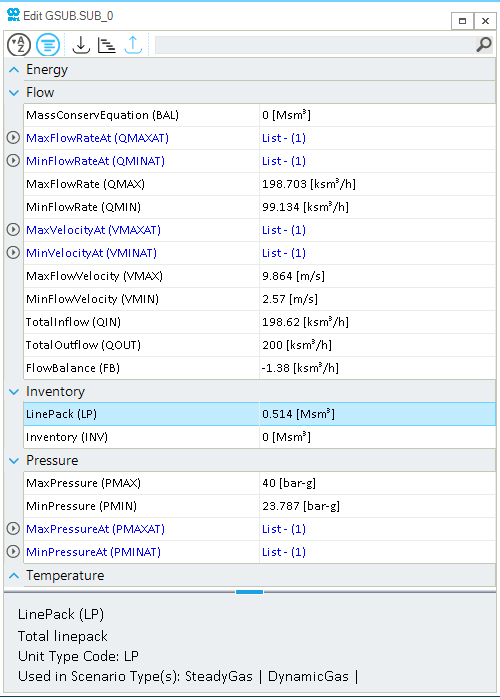
3. Property editor results tab

Alternatively, you can analyze the network or object results using the property editor’s results tab. You will analyze some results at the sub-network level using the property editor. Right-click the GSUB.SUB_0 object under Subs from the model explorer to access the context menu. Select Open Editor from the context menu. A sub-network property editor appears on the screen, as shown in Figure 5.

Figure 5. Gas subnetwork editor

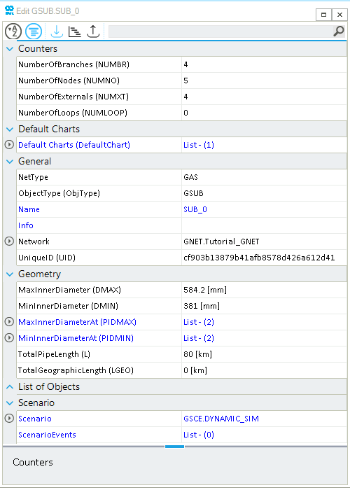
In the property editor, scenario input properties and results are displayed based on the display time of the map window. Access the results tab by clicking on the bt02 step02 06 button from the toolbar of the property editor. The expandable sections in the property editor table belong to a particular category of input properties and results. Collapse the categories Energy and Temperature as you have not covered these two aspects anywhere in the beginner tutorials. Figure 6 shows the main results for the subsystem, like the total linepack. The values you see correspond to the last time step of the simulation, which is aligned with the display time of the map window. But you can use the time function to set it to any moment.

Please, note that in this case, there is only one subsystem. So, there is no difference between it and the entire system.

Figure 6. Gas subnetwork editor with scenario results.