Step 5: Run the Steady State Simulation
In previous tutorial sections, you created all the elements needed to build a hydraulic gas model in SAInt. This step will focus on running a steady state simulation, checking the simulation log, and exploring the results using the object labels.
1. Execute the scenario
You have done all the hard work and are ready to run your scenario assuming steady state conditions for the tutorial gas network. Go to the simulation tab and press Gas. During the scenario execution, you can track the progress by observing the status bar at the bottom of the screen. Additionally, the log window will display the simulation progress during each consecutive run. Once the simulation has finished, a prompt will appear with the message "SteadyGas simulation completed successfully!". Close the window by pressing OK.
|
If the scenario execution fails, please review the previous steps and ensure everything is correctly defined. If the problem persists, please do not hesitate to contact the encoord support team for guidance. |
2. The log of the simulation
The log window is the first place to check when your simulation has problems or cannot be solved. SAInt keeps track of the status of the solver and informs the users of constraint violations, changes in the control mode of facilities, and, ultimately, failures. When no red lines are there, your simulation is successful. So, congratulations! Any condition preventing the simulation from finishing is summarized in the error message but must always be considered together with the actions taken by SAInt to deal with constraint violations (any yellow line in the log).
Light green lines inform the user on how the solver is progressing in solving the underlying mathematical problem and the convergence. Dark green lines describe the type of simulation, the model’s overall structure, the type of equation used to address the pipeline flow, or the reference conditions used for temperature and pressure. Also, the log reports default gas properties, the gas quality, and the status of temperature tracking.
SAInt always informs the user of the total computing time. So you can manage your coffee breaks!
|
The user is warmly encouraged to go through the log at the end of each simulation. This habit helps understand the simulation’s performance and to be confident in the results' accuracy. |
3. Explore results with labels and the map window legends
The fastest way to explore the results of a steady state simulation is to check the pressure and flow values at some key points. You can inspect your system by using the labels you have set for the nodes and the control valve (see Figure 1). As expected, the flow at the supply point is equal to the sum of all demand exits (i.e., 200 ksm3/h). The drop in pressure from the supply point to GNO.NODE3 is almost 5 bar-g (from 40 to 35.06 bar-g). While the pressure at GNO.NODE5 is around 23.70 bar-g.
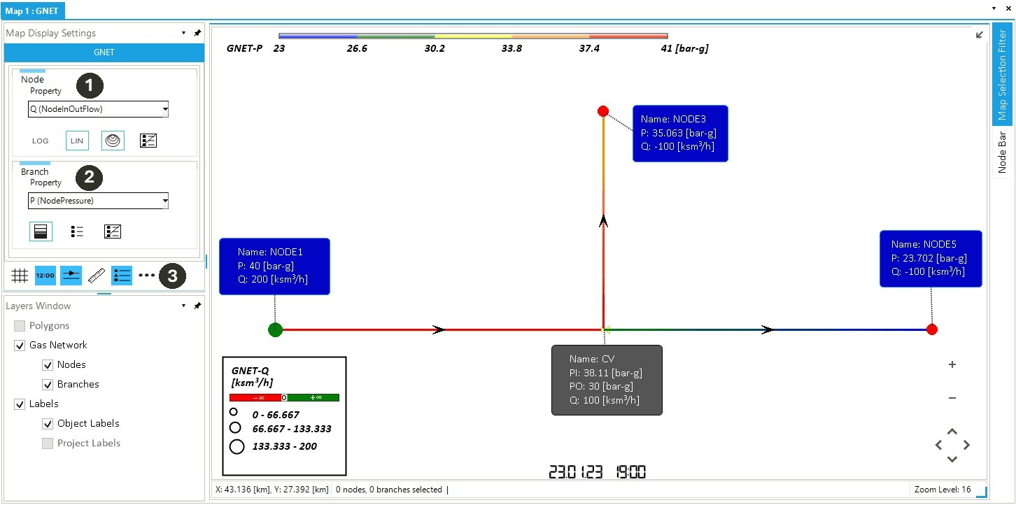
Another way to visualize the results for the entire network is to use the appearance of nodes and pipelines based on the value of a specified property. You can change which property you want to associate with the size of your nodes (❶ in Figure 1) from the node property legend, as well as the size should be scaled using a linear or a logarithmic scale. You can easily change the displayed branch property as well by using the branch property legend drop-down menu (❷ in Figure 1). You can customize the number, the color, and the size of the classes defining the legend. Access the rich color legend setting interface by clicking the dedicated button (❸) in the map view.