Scenario

A scenario is a case study performed on a network. It is characterized by a type (e.g., SteadyGas, Steady ACPF, QuasiDynamic ACOPF, DCUCOPF, etc.), a length (i.e., a starting and ending time), a definition of settings, controls, and constraints, and their behavior over time (i.e., how they change by means of events and profiles). The mathematical model describing the type of scenario can be either a simulation or an optimization problem.

Please, refer to the How-To "Create a Scenario in SAInt-GUI" for more details on how to develop your own scenario in SAInt.

The sections "Gas Scenarios", "Electric Scenarios", and "Thermal Scenarios" provide mode details on the specific type of scenario. The section "Scenarios and Hub Systems" describes the special case of combined systems.

1. General properties

A scenario has a set of specific properties editable via the scenario editor. The scenario editor can be accessed using the ESCE, GSCE or TSCE under the scenario tab. The type of button depends on the type of available networks (e.g., electric, gas, or thermal). All scenario types in SAInt have a set of identical general properties. Table 1 provides an overview of the general properties of a scenario. The following section describe more specific properties of a scenario.

Table 1. General properties of a scenario. The properties `IniState` and `Info` are editable.
Property	Description
`Network`	Name of the network the scenario belongs to
`SolverStatus`	Current status of the solver for the active scenario (e.g., solved, failed, etc.)
`Name`	Name of the scenario
`SceType`	Type of the active scenario (e.g., DCUCOPF, etc.)
`IniState`	Name of scenario whose terminal state is used as an initial state for the active scenario. "NONE" is used as default initial state if no other scenario is specified.
`Info`	Optional information the user can specify related to the active scenario

1.1. Chart properties

It is possible to specify the time interval of interest for charting the results of a scenario. The chart section of the property editor allows to define the chart time window (i.e., by specifying ChartStartTime and ChartEndTime) of all the plots generated for the active scenario. For example, if a scenario has a time window of 1 year, but the user is interested in a specific week, it is possible to specify the time interval and generate only charts displaying results only for that specific week. A different chart time step (ChartTimeStep) compared to the scenario time step can also be defined. Table 2 provides an overview of the properties of the chart section.

Table 2. Chart properties of a scenario.
Property	Description
`ChartStartTime`	Start time for all chart plots
`ChartTimeStep`	Time step for all chart plots. It can be different form the time step of the simulation or optimization.
`ChartEndTime`	End time for all chart plots

1.2. Profile properties

The dynamic behavior of many events in a scenario can be modulated by using profiles. The profile section of the property editor of the active scenario allows to fine-tune how profiles are used. The profile properties allows to decide if to use a common global start time for all profiles (GlobalProfileStartTime) and to specify the exact starting time (GlobalProfileStartTime). Alternatively, the GlobalProfileStartTime is overridden by the individual profile start time (PrfStartTime). For example, if the GlobalProfileStartTime is 01/01/2022 01:00 while the PrfStartTime is 01/01/2022 05:00 for a PSET event on an EDEM object, the profile will start according to the PrfStartTime if GlobalProfileStartTime is unchecked.

Furthermore, it is possible to use an average profile for an event in place of the original profile by checking the option AverageFlowProfiles. The AverageFlowProfiles replaces the profile values with a moving average computed between a pair of adjacent scenario time steps. For example, if the first three values of a profile are 240, 234, and 228, the average flow profile will be 240, 237, and 231. The first data point of a profile is never averaged. Table 3 provides an overview of the properties of the profile section.

Table 3. Profile properties of a scenario.
Property	Description
`UseGlobalProfileStartTime`	Enables or disables the use of the global profile start time for all profiles. The default is to have the option checked (i.e., Boolean value set to true). If unchecked, each profile is applied based on the time specified in `PrfStartTime`.
`GlobalProfileStartTime`	Set the start time for all profiles included in the active scenario. The default value is to match the start time of the scenario. The option is considered only if `UseGlobalProfileStartTime` is set to true.
`AverageFlowProfiles (AverageFlowPrf)`	Indicates if all flow properties (unit per time) with an assigned profile should use an averaged profile over the scenario’s time steps. The first data point of a profile is never averaged.

1.3. Other properties

The property editor allows to access and modify other properties associated with the active scenarios. In the time section of the property editor, the user can modify the start time and the end time of the scenario, as well as the time steps. Or in the solver section, the user can review the main settings of the solver for the simulation or optimization problem addressed by the active scenario. Please, refer to the section "Gas Scenarios", "Electric Scenarios", and to the section "Thermal Scenarios" for more details.

The section "File Information" of the property editor covers details concerning the version of SAInt used to create the scenario, the time of creation and the time the scenario was last modified, and, finally, the path to the scenario file on the computer. The section list of objects allows the user to see and modify the list of profiles associated with the active scenario. While the section network provides details on the type of network, its name, and path to the file.

2. Scenario events

A key component in a scenario is an "event". An event defines a change in the setting, control, or constraint of a property of an object in the network at a specific time during the execution of a scenario. An object in a dynamic scenario can have multiple scenario events, listed in the collection editor for scenario events. In a steady state scenario objects are generally associated to one event of each type. The user can visualize and modify events either for a single object using the option "filter scenario event" or for the scenario using the scenario table. For a single object, the list of all events associated with the object is accessible by selecting the filter scenario events option from the context menu of the object. An event can simultaneously be created for multiple objects, as long as the objects are of the same type. An easy way to select objects of the same type is by using the model explorer window.

The list of all scenario events can be visualized from the event table, accessible using the EEVT, GEVT or TEVT under the scenario tab. An example of an instance of the "collection editor" and of an "event table" is shown in Figure 1 and Figure 2.

Please, refer to the How-To "Create a Scenario Event in SAInt-GUI" for more details on how to add your own set of events to an active scenario in SAInt.

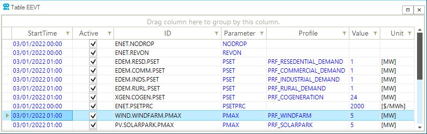
Figure 1. Example of a collection editor for an XGEN object.

Figure 2. Example of an electric scenario events table.

In the "event table", similar to the property editor and other windows in the SAInt-GUI, all text in blue can be edited by the user, while all text in black is fixed and can not be changed.

There are four scenario events categories common to all types of networks: set point, constant-updating, state, and constraint events. For electric networks, SAInt has a fifth category of events the average event. All scenario events are characterized by a common set of properties described in Table 4.

Table 4. List of the properties of all types of events.
Property	Description
`StartTime`	Start time of the scenario event. For steady state scenarios, the value is set to the start time of the scenario. For dynamic scenarios, the value can be expressed either by a specific time (e.g., dd/MM/yyy hh:mm) or by indicating the number of hours and minutes to add to the starting time (e.g., +hh:mm).
`Parameter`	Scenario event parameter (e.g., `PSET`, `QSET`, etc.). Events depend on the object type.
`Value`	The scenario event value can be either a numeric value or an arithmetic expression. If a profile is assigned to the event, the value is used to scale the profile value at a specific time (e.g., 5, -3.2, `EDEM.NAME.PSET`, etc.).
`Unit`	The unit of measure to be used for the value of the event. This unit can be different from the default units of measure for the project. A drop-down menu allows selecting a different unit within the same unit type.
`Active`	Indicates if a scenario event is active (i.e., true) or inactive (i.e., false). Inactive events are not evaluated during the execution of the scenario.
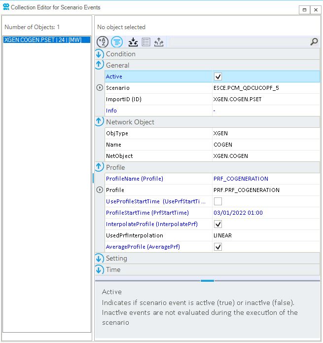
`ProfileName (Profile)`	Name of the profile assigned to the scenario event
`UsePrfStartTime (UsePrfStartTime)`	Indicates if the profile start time defined for the event should be used instead of the global profile start time defined for the scenario
`ProfileStartTime (PrfStartTime)`	Start time of the first data point of the assigned profile. The default is to have the same global start time for all events in the active scenario. It could be modified on an event base by the user.
`InterpolateProfile (InterpolatePrf)`	The user can specify if an event value is modified by a profile only at the exact moment specified by the profile or for any time point where the profile is not defined. In this case, the profile is interpolated. It is a Boolean value with a default set to true.
`AverageProfile (AveragePrf)`	Indicates if profile values should be averaged over a scenario time step. The default is set to false. The option is considered only if `InterpolateProfile (InterpolatePrf)` is set to true.
`UsedPrfInterpolation`	Defines which profile interpolation type is used for interpolating the data points included in the profile. If no profile is assigned to the event, the value is "NOPRF". Other accepted values are: "POINT" for no interpolation between two data points, "STEP" for step interpolation, "LINEAR" for linear interpolation, and "CUBIC" for cubic splines interpolation. The interpolation allows to have a different time granularity between profiles and simulation.
`Condition`	Logical expression returning a true or false value. A script editor can be accessed to evaluate the expression.
`Evaluation`	Evaluation type for the logical expression defined for the condition property. Default value is "NONE". Accepted values are: DoIFTrue, DoIFFalse, DoUtilTrue, and DOUntilFalse. The expression is evaluated if it is true or false, or until the condition is true or false.
`Name`	Name of the object to which the event is associated
`ID`	Unique identification code for the object to which the event is associated
`Info`	Optional information defined by the user for the event
`ObjType`	Code of the type of object to which the event is associated

StartTime is only applicable to dynamic or quasi-dynamic scenarios.
If the profile is assigned to an event, the Value is scaled by multiplying by the profile weight for the active time step.
An event without a profile applies only at the StartTime and after that it is constant.
Some properties for an event may not be present in the scenario table. Use the "choose columns" or "show all columns" option to display the missing properties.

2.1. Set point event

A set point event is a desired value prescribed for a variable in the mathematical model describing a scenario. Figure 3 shows an example of a set point event for the penalty price (PSETPRC) of an electric demand (EDEM) object.

Figure 3. Example of a set point event in the case of an electric demand (EDEM) object.

2.2. Constant-updating event

A constant-updating event uses a profile to update the value of an object property for every timestep. Figure 4 shows an example of a constant-updating event for the power set point (QSET) of a gas demand (GDEM) object. The profile associated with the event has as name "PROFILE1" and it uses a cubic interpolation for time steps between profile points. Data interpolation is active, and the start time is set to the global scenario start time.

Figure 4. Example of a constant-updating event.

If the data points of a profile are less than the scenario time steps, profile data is interpolated by default.

2.3. State events

The state events have three types:

ON event: An ON event indicates that the network object is active and working. The solver is forced to include the object in the simulation/optimization. Figure 5 shows an example of an ON event for a solar generator (PV) at the time step 07/09/2022 00:00. The ON event is different from the status InService, because it the equation of the object is incorporated in the mathematical problem. When InService is "FALSE", the equation is not considered, the problem is simpler, and no events can be associated to the object.

Figure 5. Example of an ON event.

OFF event: An OFF event indicates that the network object is out of service. The solver is forced to exclude the object from the simulation/optimization. Figure 6 shows an example of an OFF event for a solar generator (PV) at the time step 01/01/2022 00:00. In (quasi-)dynamic problems other events may be associated to the object at different times.

Figure 6. Example of an OFF event.

ONOFF event: An ONOFF event indicates that the network object can be put back in service. The solver is evaluating if the object should be included or excluded in the simulation. Figure 7 shows an example of an ONOFF event for a fuel generator (FGEN) from 12/01/2022 00:00.

Figure 7. Example of an ONOFF event.

2.4. Constraint events

A constraint event sets the upper and lower limit of a variable. Figure 8 shows an example of a constraint event for the available capacity of a fuel generator (FGEN) from 10/01/2022 01:00.

Figure 8. Example of a constraint event.

2.5. Average events

An average event creates an additional constraint on an electric object, which limits the average value of the object property over the time horizon of the scenario in the electric network. The averaging period of the event is defined from the following timestep after the event start time until the end time horizon. Additionally, an averaging period can be limited if another event is defined during this period. The average events have three sub-categories:

PAVG event: A PAVG event defines an average constraint on the active power (P) of an electrical demand object (EDEM) for the defined averaging period. Figure 9 shows an example of a PAVG event to constrain the active power of the electrical demand object during a 24-hour time horizon. In this example, the averaging period is from 18/07/2022 01:00 until 19/07/2022 00:00.

Figure 9. Example of a PAVG event.

FAVG event: A FAVG event defines an average constraint on the fuel consumption rate (F) of a fuel object (FUEL) for the defined averaging period. Figure 10 shows an example of a FAVG event to constrain fuel consumption of the fuel object during a 120-hour time horizon. In this example, the averaging period is from 18/07/2022 01:00 until 23/07/2022 00:00.

Figure 10. Example of a FAVG event.

AvgUpBound and AvgLowBound event: An AvgUpBound and AvgLowBound, also called multi-temporal constraints, are average events which define an upper and lower average constraint on the value of an electric variable (EVAR) for the defined averaging period. Figure 11 shows an example of an AvgUpBound event to constrain the active power of a set of hydro generators (HGEN) objects during a set time interval. In this example, the averaging period is from 18/07/2022 07:00 until 18/07/2022 19:00.

Figure 11. Example of an AvgUpBound event.

3. Scenario profiles

A profile is a collection of temporally equidistant data points. Profiles are assigned to object properties through events. The processing of profile data points is based on the specified profile settings. A profile can be applied to multiple events. In Figure 12, the profile "PRF_AT_DEMAND" is applied to the active power set point (PSET) of an electric demand (EDEM) and to the minimum value (MinVal) required by an ancillary service (ASVC).

Figure 12. Example of use of a single profile with multiple events.

The list of all profiles associated with the scenario can be visualized by the "profile table", accessible using the EPRF or GPRF under the scenario tab. As shown in Figure 13, the "profile table" is separated into three sections:

[1] "profile description table" displays the list of all the profiles and their properties.
[2] "profile data table" provides the selected profile’s mean and deviation data points list. Deviation data is only used for stochastic profiles.
[3] "profile chart window" visualizes the selected profile’s data points against the scenario time window.

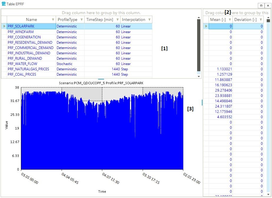
Figure 13. Example of electric scenario profile table.

Table 5 provides an overview of all relevant properties of profiles.

Table 5. Profile properties.
Property	Description
`Name`	Name of the profile
`Info`	Additional user specified information related to the profile
`ProfileType`	Type of the profile. SAInt accepts either deterministic or stochastic profiles. In deterministic profiles, the default type, the data points are specified and unchanged during the simulation. In stochastic profiles, data points are randomly generated each time a scenario is executed.
`TimeStep`	The time interval between two consecutive data points. The unit of measure is specified in the project settings.
`Interpolation`	The interpolation type used when generating profile values between two data points. Available options are linear (default), cubic, and step interpolation.
`BaseDev`	The standard deviation applied to all data points in stochastic profiles. Only used if `UseBAseDev` is selected.
`MaxVal`	The upper bound for profile values. The default value is infinite.
`MinVal`	The lower bound for profile values. The default value is negative infinite.
`DevAtMax`	Enables or disables the use of the standard deviation if the mean of the profile data is equal to `MaxVal`
`DevAtMean`	Enables or disables the use of the standard deviation when generating profile values for time points equal to the profile data point. If disabled, the deviation is only applied for profile time points where interpolation is required.
`DevAtMin`	Enables or disables the use of the standard deviation if the mean of the profile data is equal to `MinVal`
`Distribution`	Indicates which probability distribution function to use when generating profile values for a stochastic profile. Options are uniform (default), normal, or exponential distribution.
`Duration`	Indicates how profile values generated for time points outside the profile time window should be treated. The profile time window is derived by multiplying the time step by the number of data points. Available options are periodic (default), constant, and stop. Option periodic repeats the profile. Constant uses a constant profile value equal to the last data point value. And stop sets the profile value to zero.
`Points`	Number of data points in the profile
`Sign`	If enabled negative profile values are considered, otherwise negative values are set to zero
`UseBaseDev`	Option to use the same standard deviation `BaseDev` for all data points. Default value is false (i.e., unchecked).
`UseBounds`	Enables or disables the use of `MaxVal` and `MinVal` as upper and lower boundaries when generating profile values. It applies to both deterministic and stochastic profile types.
`ProfileDataPoints`	Collection of profile data points. The user can add, edit, or remove points. This option is represented as a small, separated table in the profile table window.
`Scenario`	Name of the scenario to which the profile is assigned. This option is available in the property editor of a profile.

Please, refer to the How-To "Create a Profile in SAInt-GUI" and "Assign a Profile to an existing Event" for more details on how to use profiles in your scenario.

3.1. Profile type

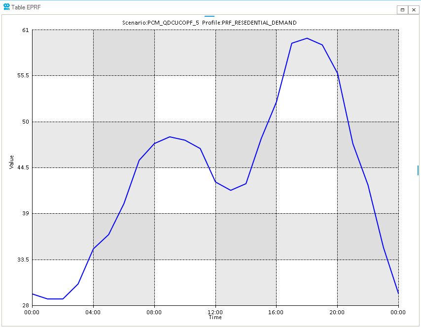
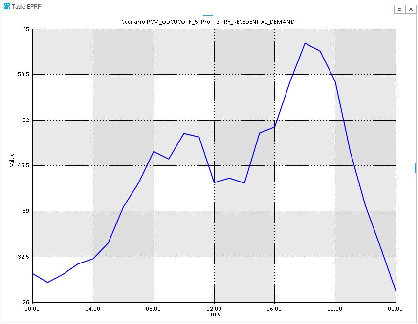
SAInt accepts two types of profiles: deterministic and stochastic profiles. In deterministic profiles, the default type, the user must define a priori the value of all data points. Such figures are not automatically changed between the simulation. In stochastic profiles, data points are randomly generated each time a scenario is executed. New values are sampled based on the type of distribution selected (i.e., uniform, normal, or exponential), and on the specified mean and standard deviation. Figure 14 shows an example of a deterministic profile, while Figure 15 shows an example of a stochastic profiles using the deterministic as mean value and setting a uniform distribution with standard deviation equal to 20.

Figure 14. Example of a deterministic profile.

Figure 15. Example of a stochastic profile.

3.2. Profile distribution

Stochastic profiles are defined by specifying the mean and standard deviation value for each profile data point, along with the type of random distribution to be used from drawing random samples. SAInt allows the user to select one of the three distribution options for the Distribution property. We have:

Uniform distribution: It applies a uniform probability distribution;
Normal distribution: It applies a normal probability distribution;
Exponential distribution: It applies an exponential probability distribution.

3.3. Profile interpolation

The time granularity of a profile and of a scenario may differ. When a profile has a coarser granularity, the user can specify if and how to interpolate for any time step not present in the profile. All interpolation options generate profile values between two data points. Available options are:

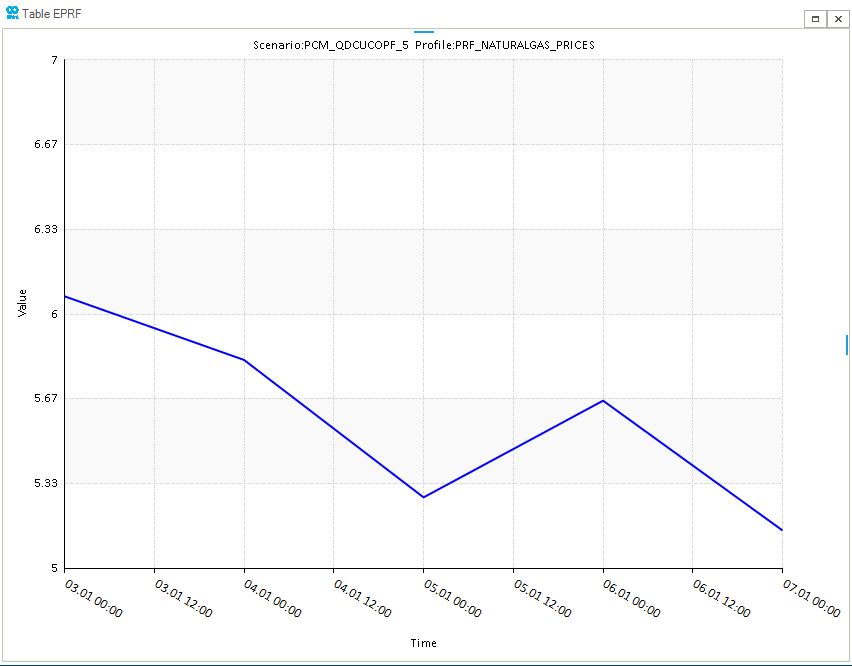
Linear interpolation: It applies linear interpolation between data points. In Figure 16, daily fuel prices of natural gas are linearly interpolated to hourly scenario time steps.

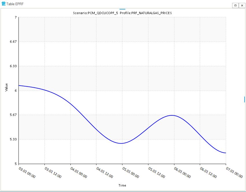
Figure 16. Example of linear interpolation.

Cubic interpolation: It applies cubic interpolation between data points. In Figure 17, daily fuel prices of natural gas are interpolated using a cubic model to hourly scenario time steps.

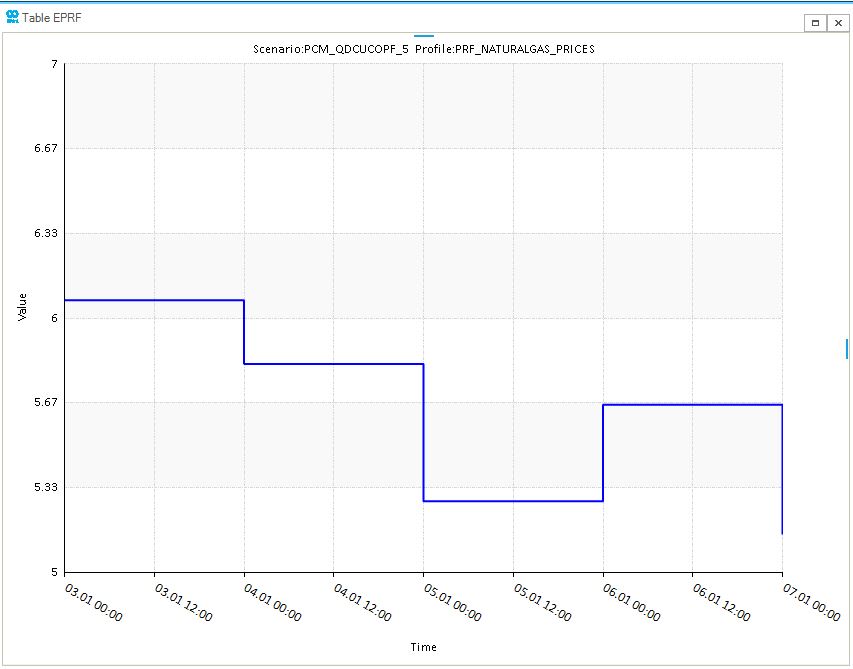
Figure 17. Example of cubic interpolation.

Step interpolation: It applies step interpolation between data points. In Figure 18, daily fuel prices of natural gas are interpolated using a step model to hourly scenario time steps.

Figure 18. Example of step interpolation.

3.4. Profile duration

The length of a profile is defined by the number of data points multiplied by the time step. When a scenario has a length greater than the one of a profile, it is necessary to extend a profile so as to cover the entire simulation or optimization problem. Available options for the Duration property are:

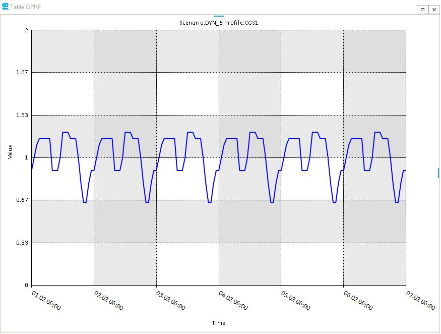
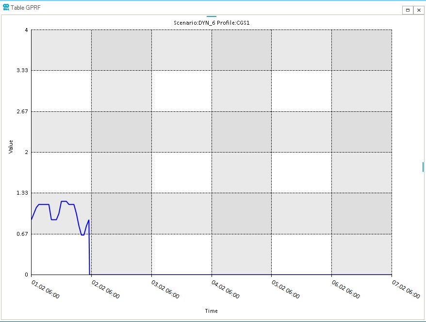
Periodic: It repeats periodically the profile. In Figure 19, the profile is only defined for 24 hours. After the defined values, the profile is periodically repeated based on the length of the profile or fractions (i.e., 24 data points).

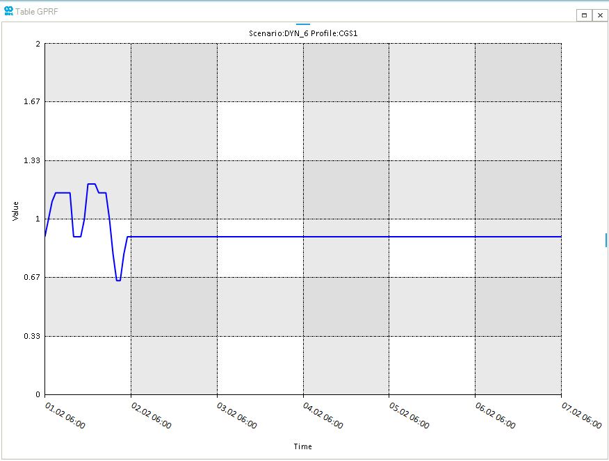
Figure 19. Example of a periodic profile.

Constant: It creates a constant profile equal to the last data point value. In Figure 20, the profile is only defined for 24 hours. After the defined values, the profile is extended with a constant value.

Figure 20. Example of a constant profile.

Stop: It sets the profile value to zero. In Figure 21, the profile is only defined for 24 hours. After the defined values, the profile is set to zero.

Figure 21. Example of a stop profile.