Graph Functions
This section describes the graph functions available in SAInt. These functions are used to analyze and aggregate object input properties and output results to understand their behavior. The function returns data already formatted for a table or plot function so to create out-of-the-box tables or charts. All functions starts with the prefix "g" to stress the need of a graphical output in the form of a table or chart.
The functions are listed in Section 1 with their syntax, description, and output examples. The syntax of the functions includes expr which refers to the input expression. The examples shown are based on the dynamic scenarios of the sample electricity (ENET09_13) and gas (GNET29_18) networks available in the user’s Projects folder (C:\...\Documents\encoord\SAInt-v3\Projects). Please consider the type of object used in the expression to select the correct network. Scenario results must be available for the expression to be executed correctly in the command window. Note that the sample electricity (ENET09_13) model uses a stochastic profile for the hydro reservoir. This is why the user may get different results from the ones presented here or each time the same command is used in the active session of SAInt.
The user can easily copy and paste the code in the command window and replicate the examples.
1. Graphical functions description
The graphical functions work with an expression selecting multiple objects of the same type. They perform a task on the set of property values for a certain time step given multiple objects.
As an example, check the expression of the function gsum. The form of th expression is GSUP.%.Q.(%), which reads like "select all external of type supply and extract the flow for each time step". SAInt will build a matrix with the number or rows defined by the number of time steps, and the number of columns equal to the number of supply points. The function gsum will calculate the sum over the rows.
1.1. The function gsum
gsum('expr')
Returns a data series representing the sum of the values of a property for a set of objects evaluated by the specified input expression.
Examples:
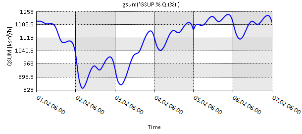
plot(gsum('GSUP.%.Q.(%)'))-
Plots the data series containing the sum of flows from all gas supplies at each time step of the simulation.
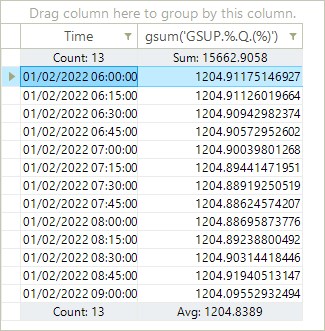
table(gsum('GSUP.%.Q.(%)'), '01/02/2022 06:00', '01/02/2022 09:00')-
Tabulates the data series containing the sum of flows from all gas supplies at each time step of the simulation. To restrict the output a start and end time are specified for the
tablefunction.
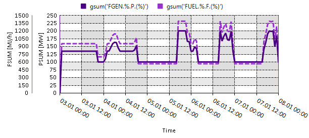
nplot(gsum('FGEN.%.P.(%);3;indigo;[250,0,10]'), gsum('FUEL.%.F.(%);3;dash;darkorchid;[1500,0,10]'))-
Plots two data series in a single chart. The first data series is the sum of active power from all fuel generators at each simulation time step. The second data series is the sum of fuel consumption from all fuels at each simulation time step.
1.2. The function gabssum
gabssum('expr')
Returns a data series representing the sum of the absolute values of a property for a set of objects evaluated by the specified input expression.
Examples:
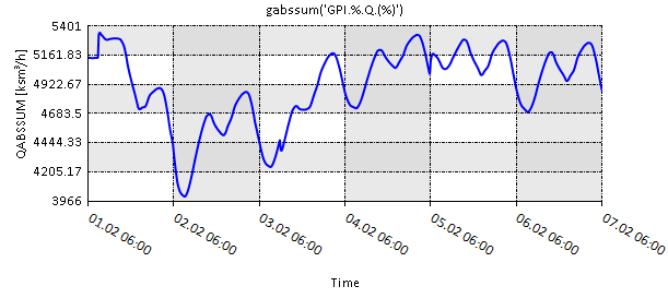
plot(gabssum('GPI.%.Q.(%)'))-
Plots the sum of absolute values of gas flows through all gas pipelines at each time step of the simulation.
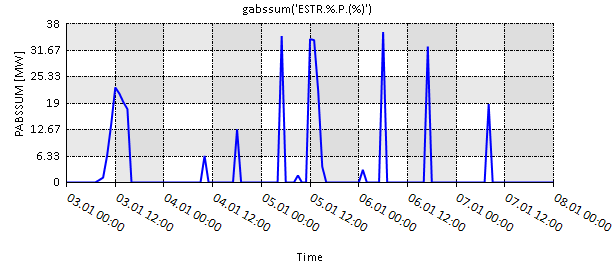
plot(gabssum('ESTR.%.P.(%)'))-
Plots the sum of absolute values of power generated or consumed by all electric storages at each time step of the simulation.
1.3. The function gmean
gmean('expr')
Returns a data series representing the mean of the values of a property for a set of objects evaluated by the specified input expression.
Examples:
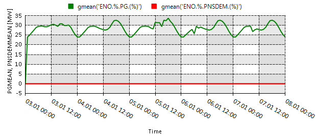
nplot(gmean('ENO.%.PG.(%);green;[35,-5,8]'), gmean('ENO.%.PNSDEM.(%);red'))-
Plots two data series in a single chart. The first data series is the mean active power generated at all electric nodes at each time step of the simulation. The second data series is the mean power not served at all electric nodes at each time step of the simulation.
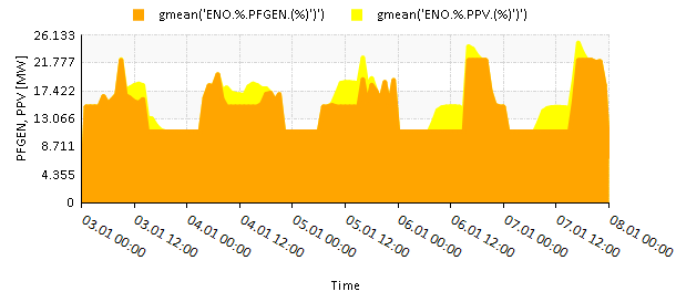
stackplot(gmean('ENO.%.PFGEN.(%);orange'),gmean('ENO.%.PPV.(%);yellow'))-
Creates a stack plot of the mean power generated by all fuel generators and solar plants at all electric nodes, at each time step of the simulation.
1.4. The function gabsmean
gabsmean('expr')
Returns a data series representing the mean of the absolute values of a property for a set of objects evaluated by the specified input expression.
Examples:
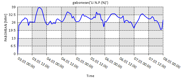
plot(gabsmean('LI.%.P.(%)'))-
Plots the mean of absolute transmission flows through all electric lines at each time step of the simulation.
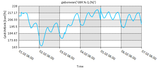
plot(gabsmean('GBR.%.Q.(%);deepskyblue'))-
Plots the mean of absolute flow values through all gas branches at each time step of the simulation.
1.5. The function gdev
gdev('expr')
Returns a data series representing the sample standard deviation of the values of a property for a set of objects evaluated by the specified input expression.
Example:
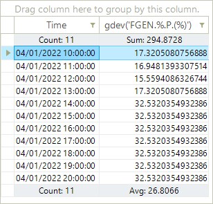
table(gdev('FGEN.%.P.(%)'),'04/01/2022 10:00','04/01/2022 20:00')-
Tabulates the sample standard deviation of the power generated by all fuel generators at each time step of the simulation within a start and end time. As an example, check the value calculated for the time step 04/01/2022 10:00 and the one you can derive by looking at the value from the expression
FGEN.%.P.(34).
1.6. The function gabsdev
gabsdev('expr')
Returns a data series representing the sample standard deviation of the absolute values of a property for a set of objects evaluated by the specified input expression.
Example:
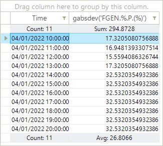
table(gabsdev('FGEN.%.P.(%)'),'04/01/2022 10:00','04/01/2022 20:00')-
Tabulates the sample standard deviation of the absolute power generated by all fuel generators at each time step of the simulation within a start and end time.
1.7. The function gmax and gmin('expr')
gmax('expr') and gmin('expr')
These functions return a data series representing, respectively, the maximum and the minimum of the values of a property for a set of objects evaluated by the specified input expression.
Examples:
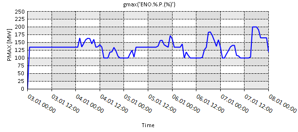
plot(gmax('ENO.%.PNS.(%)'))-
Plots the maximum power not served at all electric nodes at each time step of the simulation.
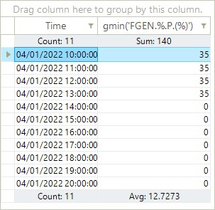
table(gmin('FGEN.%.P.(%)'),'04/01/2022 10:00','04/01/2022 20:00')-
Returns a table, bounded within a start and end time, with two columns:
- First Column
-
Consists of rows with each time step of the simulation.
- Second Column
-
Consists of rows with the minimum power generated from all fuel generators at each time step of the simulation.
1.8. The function gabsmax and gabsmin('expr')
gabsmax('expr') and gabsmin('expr')
These functions return a data series representing, respectively, the maximum and the minimum of the absolute value of a property for a set of objects evaluated by the specified input expression.
Example:
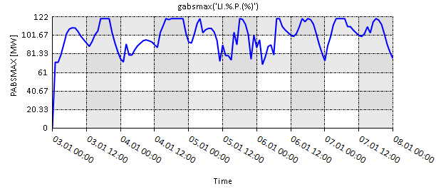
plot(gabsmax('LI.%.P.(%)'))-
Plots the absolute values of maximum power flow through all electric lines at each time step of the simulation.
1.9. The function gmaxat and gminat('expr')
gmaxat('expr') and gminat('expr')
Returns a list of objects representing where is the maximum or the minimum of the values of a property for a set of objects evaluated by the specified input expression.
Example:
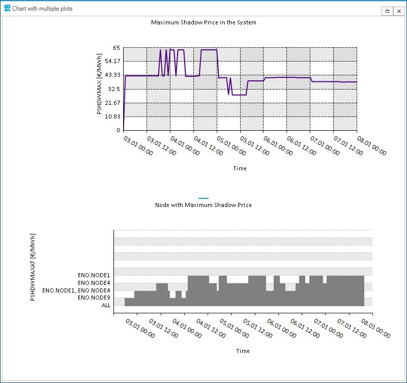
subplot(plot(gmax('ENO.%.PSHDW.(%);indigo;title=Maximum Shadow Price in the System')),plot(gmaxat('ENO.%.PSHDW.(%);Gray;column;Title=Node with Maximum Shadow Price')))-
Creates a chart window with two plots. The first plot shows the maximum shadow prices in all of the nodes in the system at each time step of the simulation. The second plots shows which nodes in the system have the maximum shadow price at each time step of the simulation.
1.10. The function gabsmaxat and gabsminat('expr')
gabsmaxat('expr') and `gabsminat('expr')
Returns a list of objects representing where is the maximum or the minimum of the absolute value of a property for a set of objects evaluated by the specified input expression.
Example:
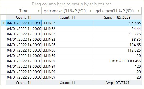
table(gabsmaxat('LI.%.P.(%)'),gabsmax('LI.%.P.(%)'),'04/01/2022 10:00','04/01/2022 20:00')-
Creates a table, bounded within a start and end time, with three columns:
- First Column
-
Consists of rows with each time step of the simulation.
- Second Column
-
List of transmission lines with the maximum power flow at each time step of the simulation.
- Third Column
-
The maximum power flow among all transmission lines at each time step of the simulation.