Dock Panel

The section describes the controls and options included in the dock panel of SAInt-GUI. The dock panel consists of (Figure 1):

the project explorer (1): to manage all the file resources related to the active project.
the model explorer (2): to access objects and model-related data of the networks in the project.
the map window (3): to display a network, scenarios, and results in tabular form.
the script editor (4): to develop scripts in IronPython to interact with the model and the results.
the property editor (5): to display the full set of properties of a selected object.
the workspace (6): to have a list of functions to be used in the command window or in an IronPython script.
the command window (7): to interact with SAInt core using a command line interface.
log window (8): to record and log actions performed by SAInt and simulation or optimization messages.
the chart window (9): to display charts of properties and results.

The elements of the dock panel can be controlled either at the element level or from the entry View of the ribbon bar (see number 10 in Figure 1).

Figure 1. Main elements of the dock panel of SAInt-GUI. Numbers indicate: (1) the project explorer, (2) the model explorer, (3) the map window, (4) the script editor, (5) the property editor, (6) the workspace, (7) the command window, (8) log window, and (9) the chart window. Number (10) indicates the entry View in the ribbon bar from where the user can control the previous windows.

1. Window interaction and positioning

The SAInt graphical user interface is highly customizable. The user can activate, remove, dock, or re-arrange windows based on the specific needs of a project. The tab "View" in the ribbon bar allows users to interact with the different windows and modify the general layout easily. If a window is closed, the user can open it again from the tab View menu. Each window contains a title bar (at the top) and the main dock area. On the right side of the title bar, three buttons allow for closing the window (right-most x-shaped icon), auto-hiding the window (middle pin-shaped icon) and modifying the state of the window (left-most triangle-shaped icon) from dockable to floating or tabbed. In the case of the map window, the triangle-shaped icon provides a list of the available tab views.

The user can interact with the windows by using the mouse on the title bar and:

by holding the left button pressed

The selected window can be dragged to a new position. SAInt shows marks on the other windows to suggest docking actions and positions, like in Figure 2. The window can also be positioned on a different screen to take advantage of a multi-screen layout.

by left-clicking

The user can change the docking mode of each window to floating, dockable, hide, auto-hide, or tabbed document, as shown in Figure 3. The docking modes can be selected by using the downward arrow button (located on the right of the title bar) or right-clicking on the title bar. The available options are:

Floating: Pops out the selected window in a floating state. The user can then drag the floating window to the desired location.
Dockable: Docks the selected window to its default location on the SAInt-GUI.
Hide: Hides the selected window from the SAInt-GUI. The user can re-open the hidden window from the view tab.
Auto-hide: Auto-hides the selected window in the SAInt-GUI. The user can hover and click on the icon of the hidden window to dock it.
Tabbed: Makes a new tab for the selected window.

Figure 2. By holding pressed the left mouse button on the title bar, the user can drag around and adjust the position of the window. Marks are displayed to help the positioning.

Figure 3. By left-clicking on the triangle-shape icon of the title bar the user can change the docking mode of the window.

2. Project explorer

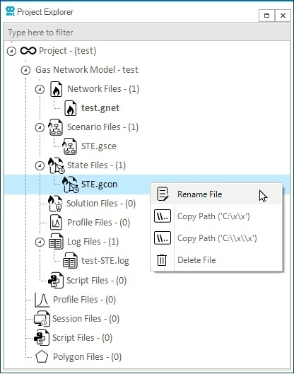
The project explorer is accessible from the project explorer tab located on the left-most window of SAInt-GUI. It gives an overview of the files available in the current project directory. Figure 4 shows an example of a gas network named "test". The project explorer has a hierarchical structure, starting from the parent entry, which indicates the current project’s name in brackets. The file types included and listed in the project explorer are:

Networks: The project explorer reports an entry for each network included in the project. This entry has a second nested level reporting: the name of the specific network, the list of scenarios for the network, the list of state and solution files for the solved scenarios, the list of profile files, the list of logs recorded after a scenario execution, and the list of script files available.
Profile files: The entry lists all the profile files in the "project" directory, which is the folder where the project file is saved.
Polygon: The entry lists all the SAInt format polygon files in the "project" directory.
Log: The entry lists all the log files in the "project" directory.
Script: The entry lists all the script files in IronPython in the "project" directory.

When right-clicking on a child of an entry, a context menu opens with a set of options allowing the user to (1) open the file with the property editor, (2) copy the path using Windows or Unix style, (3) rename the file or (4) delete the file. When a file is deleted, it is not moved to the operating system trash bin but removed from the files system. Please, remember that SAInt does not provide for an undo capability. Be careful with what you delete.

The entries in the hierarchical list can be expanded or collapsed by clicking on the triangle to the left of the entry name.

The active scenario and networks are indicated by using a bold font.

Below the title bar of the project explorer window, there is a gray text box providing searching and filtering functionalities for the files reported in the hierarchy of items.

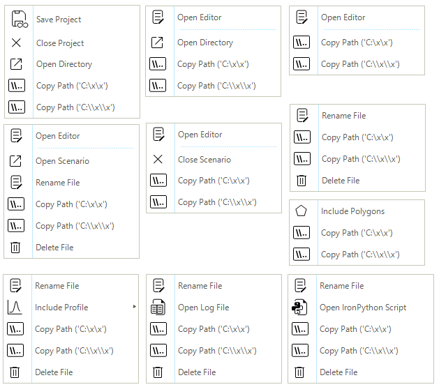
The file extension for a project file is *.prj. Only one prj file is possible in a project directory.

Figure 4. Example of the "Project Explorer" window for a gas network named test.gnet, with one scenario, one state file, and one log file. An example of a context menu is shown for the state file selected.

The entries in the project explorer have different options accessible from their context menu. Figure 5 shows examples of the context menu for different items. Other possible options are also available when the entry is active and loaded in a session. The most common operation is to copy the path to the file of the entry, load it in the active session, or delete it from the hard drive.

Figure 5. Example of the context menu for different elements of the project explorer (from top-left to bottom-right): project entry, model entry, network file, any scenario file, any state file, any solution file, the polygon entry, any profile file, any log file, and any IronPython script.

3. Model explorer

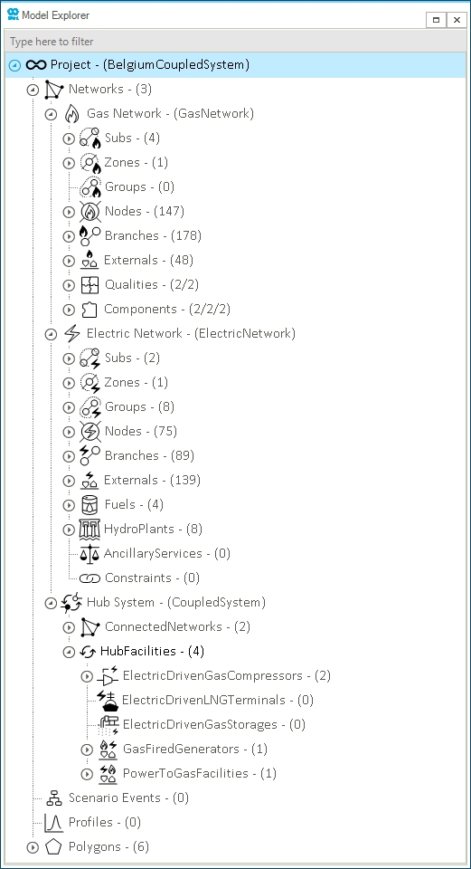
The model explorer is accessible from the model explorer tab located on the left-most window of the SAInt-GUI. It allows access to objects and model-related data of the networks in the project. Objects are presented in a hierarchical tree by object type (e.g., subs, zones, groups, nodes, branches, externals) and network type.

The model explorer is structured to show (see the example in Figure 6):

Networks: the entry provides a list of networks included in the project, and for each network, a list of subs, zones, groups, nodes, branches, or network specific objects (e.g., qualities for gas systems or fuels for electric systems). When a hub is included in the model, the entry reports the list of networks participating in the hub system and the list of hub facilities.
Scenario Events: the entry lists the events of the active scenario for each network.
Profiles: the entry lists the profiles used in dynamic simulations for each active scenario.
Polygons: the polygons loaded with the project are listed.

Clicking on the triangle to the left of a parent object name will expand or collapse the child objects.

The presence of an asterisk next to the entry name indicates that the object has not been saved yet.

The number next to a parent object’s name (e.g., branches (147) under "Gas Network" in Figure 6), indicates the total number of associated child objects. However, the numbers next to the qualities and components for a gas network give the following information:

Qualities - (1/1): The first number indicates the number of qualities assigned to gas supplies in the network, while the second indicates the number of assignable qualities.
DEFAULT - (1/1): The first number indicates the number of components with %-Mol > 0, while the second number indicates the number of components included in the supply qualities defined in the network (In this example, the defined supply quality is DEFAULT).
Components - (1/1/1): The first number indicates the number of components (e.g., methane, hydrogen) with %-Mol > 0 in at least one assignable quality, while the second number indicates the number of components with %-Mol > 0 in at least one quality assigned to a gas supply. The third number indicates the total number of available components.

Figure 6. Example of the "Model Explorer" window for a project with a gas system, an electric system, and a combined system.

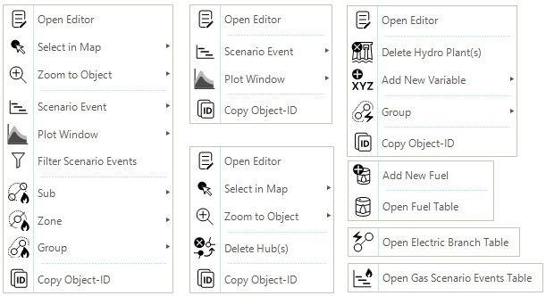
The model explorer allows quick access to object properties or functions by context menus. Right-clicking on an object (parent or child) opens the context menu. The content of the context menu depends on the type of object selected. Figure 7 shows some examples of context menus for network and scenario objects. In some cases, only one option is available, like "Open XXX Table", where XXX is the parent object container of simple objects (see examples at the bottom-right corner of the figure). In other cases, the context menu allows the user to add, remove, and modify the object and its properties. In many cases, it is possible to select the object in the map view, zoom to the object in the map view, open the property editor, or copy the object identification code. Figure 7 displays an example of a context menu for a generic generator (network mode).

Figure 7. Context menu examples for network and scenario objects.

The context menus are different when scenarios are loaded compared to the ones when only networks are loaded.

The more common context menu options for network objects, except those specific to a single network object type, are described below.

Common options

Options	Network mode	Scenario mode
Open editor(s)	Opens the object editor properties.	Opens the object editor with the filtered properties based on the scenario selected.
Open (object) table(s)	Opens the table with network-level properties.	Opens the table with network- and scenario-level properties.
Select in map(s)	Highlight the object(s) on the map window.	Highlight the object(s) on the map window.
Zoom to object(s)	Zooms to the object(s) on the map window.	Zooms to the object(s) on the map window.
Copy object-ID	Copies the object ID.	Copies the object ID.
Group Create New group	Creates the new group with the selected object(s).	Creates the new group with the selected object(s).
Sub Open Sub editor	Opens editor with network-level properties.	Opens editor with network- and scenario-level properties.
Zone Open Zone editor	Opens editor with network-level properties.	Opens editor with network- and scenario-level properties.
Plot window	Plots network level-object properties.	Plots network- and scenario-level object properties.
Scenario event(s)	-	List of events for the object(s).
Filter scenario event(s)	-	Opens the collection editor of the scenario events created for the selected object(s). The properties of the events can be changed using the editor.
Add new variable	Adds a new variable associated with the network object for a user-defined constraint. The user can select the type of variable from the secondary context menu.	-
Delete hub(s)	Deletes the selected hub facility.	-

Options

Network mode

Scenario mode

Open editor(s)

Opens the object editor properties.

Opens the object editor with the filtered properties based on the scenario selected.

Open (object) table(s)

Opens the table with network-level properties.

Opens the table with network- and scenario-level properties.

Select in map(s)

Highlight the object(s) on the map window.

Zoom to object(s)

Zooms to the object(s) on the map window.

Copy object-ID

Copies the object ID.

Group Create New group

Creates the new group with the selected object(s).

Sub Open Sub editor

Opens editor with network-level properties.

Opens editor with network- and scenario-level properties.

Zone Open Zone editor

Opens editor with network-level properties.

Opens editor with network- and scenario-level properties.

Plot window

Plots network level-object properties.

Plots network- and scenario-level object properties.

Scenario event(s)

List of events for the object(s).

Filter scenario event(s)

Opens the collection editor of the scenario events created for the selected object(s). The properties of the events can be changed using the editor.

Add new variable

Adds a new variable associated with the network object for a user-defined constraint. The user can select the type of variable from the secondary context menu.

Delete hub(s)

Deletes the selected hub facility.

Furthermore, there are set of object-specific context menus with different entries based on the node, branch, or object type. Check the following for details.

Additional options - Nodes

Options	Network mode
Add new external	Adds a new external connection to the node. The user can select the external (e.g., WIND, PV, FGEN, GSUP) from the secondary context menu.
Zone Create new zone	Creates a new zone with the selected node.
Zone Add node to (network) zone	Adds the selected node to a selected zone. The zones can be selected from the secondary context menu.

Options

Network mode

Add new external

Adds a new external connection to the node. The user can select the external (e.g., WIND, PV, FGEN, GSUP) from the secondary context menu.

Zone Create new zone

Creates a new zone with the selected node.

Zone Add node to (network) zone

Adds the selected node to a selected zone. The zones can be selected from the secondary context menu.

Additional options - Branches

Options	Network mode
Delete Branch(es)	Deletes the branch(es).
Change branch direction	Flips the direction of the branch.

Options

Network mode

Delete Branch(es)

Deletes the branch(es).

Change branch direction

Flips the direction of the branch.

Additional options - Fuels

Options	Network mode
Delete fuel(s)	Deletes the fuel(s).
Add new Fuel(s)	Adds the new fuel to the current network.

Options

Network mode

Delete fuel(s)

Deletes the fuel(s).

Add new Fuel(s)

Adds the new fuel to the current network.

Additional options - Externals and Hydro plants

Options Network mode Scenario mode

Options	Network mode	Scenario mode
Add external to ancillary service(s)	Adds the external to contribute to an ancillary service.	-
Remove from ancillary service(s)	Removes the external contributing to an ancillary service.	-
Delete external(s)	Deletes the external object(s).	-
Delete hydro plant(s)	Deletes the selected hydro plant(s).	-
Collect weather data(s)	Opens the window for weather data collection for the selected object.	Opens the window for weather data collection for the selected object.
Generate profile from weather data(s)	Opens the window for profile generation based on the collected weather data for the selected object(s).	-
Generate profile from weather data and assign to event `PSET` or `PMAX`	-	Opens the window for profile generation based on the collected weather data for the selected object and assigns an event.

Add external to ancillary service(s)

Adds the external to contribute to an ancillary service.

Remove from ancillary service(s)

Removes the external contributing to an ancillary service.

Delete external(s)

Deletes the external object(s).

Delete hydro plant(s)

Deletes the selected hydro plant(s).

Collect weather data(s)

Opens the window for weather data collection for the selected object.

Generate profile from weather data(s)

Opens the window for profile generation based on the collected weather data for the selected object(s).

Generate profile from weather data and assign to event PSET or PMAX

Opens the window for profile generation based on the collected weather data for the selected object and assigns an event.

Additional options - Ancillary services and Constraints

Options	Network mode
Delete ancillary service(s)	Deletes the selected ancillary service(s).
Delete constraint(s)	Deletes the selected constraint(s).

Options

Network mode

Delete ancillary service(s)

Deletes the selected ancillary service(s).

Delete constraint(s)

Deletes the selected constraint(s).

When scenario-related entries are selected in the model explorer, some additional context menus are available.

Additional options - Scenario events and Profiles

Options Scenario mode

Options	Scenario mode
Delete event(s)	Deletes the selected event(s).
Duplicate event(s)	Duplicates the selected event(s).
Open (network) scenario events table	Opens the scenario events for the current scenario.
Include profile(s)	Opens the window to select the profile to be included in the current scenario. The profile should be in `*.prfl` format.
Open (network) profiles table	Opens the profiles table for the current scenario.
Open (network) scenario events table	Opens the scenario events for the current scenario.
Copy profile(s)	Copies the selected profile(s).
Paste profile(s)	Creates a duplicate of the last copied profile with the same name plus the underscore (_) and the number of the copied version (example: SolarProfile_1). The paste option only works in the profile section of the model explorer or profile table.

Delete event(s)

Deletes the selected event(s).

Duplicate event(s)

Duplicates the selected event(s).

Open (network) scenario events table

Opens the scenario events for the current scenario.

Include profile(s)

Opens the window to select the profile to be included in the current scenario. The profile should be in *.prfl format.

Open (network) profiles table

Opens the profiles table for the current scenario.

Open (network) scenario events table

Opens the scenario events for the current scenario.

Copy profile(s)

Copies the selected profile(s).

Paste profile(s)

Creates a duplicate of the last copied profile with the same name plus the underscore (_) and the number of the copied version (example: SolarProfile_1). The paste option only works in the profile section of the model explorer or profile table.

4. Map window

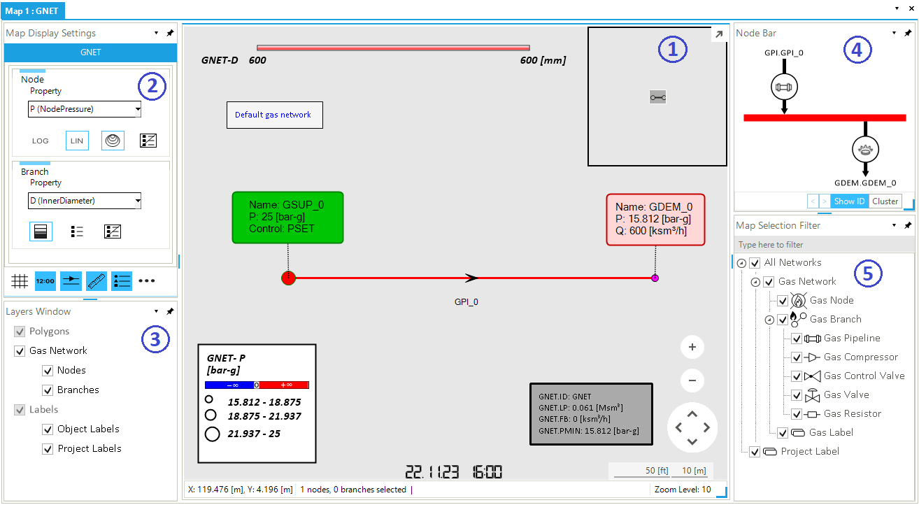
The "Map Window" is a core visualization component of SAint-GUI used to picture the geometric layout of a network, describe the topological relationships among objects, provide a geographic context with a base map, visualize property differences across a network, or show animations of solutions obtained from executing a scenario. Figure 8 shows an example of a map window where a default gas network is shown. In the example, the pipeline has a color-coded legend based on the size of the inner diameter (D) and the nodes' color and size are based on the pressure (P). Labels are used to report properties of the objects. The node bar shows details of node GNO_1 (i.e., the one on the right).

A "map window" is made of multiple parts playing a different role. We have (Figure 8):

the Map View (1): the main element of a map window is the "map view", which is the area where a network is displayed along with legends for nodes and branches, labels, zooming and panning controls, polygons, and a base map, whenever a geographic view is selected.
the Map Display Settings (2): all controls and settings for the legends of nodes' and branches' properties or results are accessible through the "Map Display Settings" window.
the Layers Window (3): the visibility of all graphical objects, like labels or polygons, and of all model objects, like branches and nodes, can be turned on/off or personalized using layers.
the Node Bar (4): it allows to see and access externals and branches connected to a selected node.
the Map Selection Filter (5): you can restrict the selection of model components or labels by turning on or off the associated type in the "Map Selection Filter".

By default, the map window is located at the center of the dock panel. When creating a new project, one map window is available, with an instance of a map view and one of the other four parts. The user can add multiple map windows in the same project, and each has its own set of parts and settings.

Figure 8. Example of a Map Window panel with (from top-left to bottom-right) the "Map Display Settings" (2), the "Layers Window" (3), the "Map View" (1), the "Node Bar" (4), and the "Map Selection Filter" (5).

4.1. Map view

The "Map View" is the component of the map window for the visualization of networks and other graphical elements like the legends, the scale bar, the labels, etc. The map view comprises a main area, where objects are placed and drawn, and a status bar at the bottom (see Figure 8).

4.1.1. Types of map view

Since the release 3.4 of SAInt, the map view has been redesigned and expanded. SAInt-GUI now has two types of map view: a Cartesian map view and a geographic map view.

The Cartesian map view is a visualization space where objects are drawn and placed in an orthonormal Euclidean system by means of X and Y planar coordinates. SAInt interprets coordinates based on the unit of measurement defined in the general settings (e.g., kilometers or miles). For any branch object where the user is required to specify the property length (L), SAInt is also calculating the property LGEO or "geographic length", derived as the sum of the length of all segments of the branch based on the Euclidean distance of the nodes or vertices using XY-coordinates.

The geographic map view is a visualization space where objects are drawn and placed in a geographic system. This system is based on an Ellipsoidal two-dimensional coordinate system, combining the World Geodetic System 1984 ensemble datum and degrees as units of measure. This reference system is known as "World Geodetic System 1984" and it is used in "global positioning system" (GPS) and by many on-line map service providers like "Google Maps", "Bing Maps", or "OpenStreetMaps". SAInt-GUI calculates the property LGEO using the "Haversine formula" in geographic map views. While coordinates are reported in degrees and fraction of a degree.

The geographic map view supports the use of a "base map". The default base map is for now taken from the open-source project OpenStreetMap. However, users can choose from two other base maps (BingMaps and GoogleMaps) and specify the preferred map service provider and the associated login credentials.

By default, SAInt provides the user with OpenStreetMap as a map service provider. OpenStreetMap is free to use under an open license. Google Maps and Bing Maps are not open-license services. They provide a variety of subscription plans for different types of users. Both map service providers offer a "free" plan for "Non-profit" and "Education" organizations.

To obtain an API key, consult the web page "Getting a Bing Maps Key" or "Getting started with Google Maps Platform" (and click on "Get Started").

The user can specify the type of map view when a new network is created by using the menu New of the tab "Network" of the ribbon bar. Or by setting the CRS of the network in the import template of any of the supported formats.

Whenever the user needs to place a network on a base map, it is mandatory to indicate the CRS used by the source data. This can be easily done by specifying the code identifying the source CRS in the field CRSType of the import template. The code value DEFAULT is for the default coordinate system used by the geographic map (i.e., WGS84 or EPSG:4326). Alternatively, the user can select the relevant EPSG code of the supported coordinate reference systems from either the information sheet of the Excel import template or from the section "Coordinate Reference Systems".

The How-To "Import data with a Coordinate Reference System" provides a step-by-step guide on how to specify the CRS in your import template.

If the user needs to work with a projected coordinate system (i.e., with a Cartesian map), there is no need to specify any CRS code, but the value NONE must be used in the field CRSType of the import template. SAINt does not perform any coordinate conversion from projected to projected reference systems. This step must be performed by the user prior to import data in SAInt.

Finally, to keep track of the original CRS, please add the EPSG code to the field Info of the *NET sheet/section of the import template.

SAInt is not meant as full-fledge cartographic software, so it allows for a reduced set of CRS and coordinates conversions. Such conversion is applied to place data on a geographic map during the import step. Or it is carried out when exporting from a geographic map to a network import file. Coordinate conversion is not possible when using a network placed on a Cartesian map view.

For details on the supported CRS refer to the section "Coordinate Reference Systems".

On a Cartesian coordinate system, we refer to the location of a point by the couple "X-coordinate (horizontal) - Y-coordinate (vertical)". On a geographic coordinate system, we refer to the location of a point by the couple "Latitude (vertical) - Longitude (horizontal)".

4.1.2. Base map types

SAInt allows the user to specify a "base map" provider to display a base map layer in a geographic map. There are three main "base map" providers available in SAInt: OpenStreetMap, BingMaps, and GoogleMaps.

To select a "base map" provider, the user can access the miscellaneous tab in the main SAInt settings window and choose a provider from a drop-down list, as shown in Figure 9. Alternatively, right-click on the entry "Base Map" of the layer window and select "Base Map Layer Settings". In the new window, it is possible to set the desired base map provider for the active map view. Each map view can have its own map provider. The user can save such choice in a session. Whenever a session is reloaded in SAInt, the settings for the base map provider for each map view are reset to the user’s selection. The option is for now valid only for the map provider and not for the type of map (i.e., aerial or base gray).

Figure 9. Select a "base map" provider in the miscellaneous tab of the settings window of SAInt.

To use "BingMaps" or "GoogleMaps", the user must provide a specific API key under the properties BingMapsAPIKey and GoogleMapsAPIKey. Only with a valid API key SAInt will be able to retrieve tile images from the BingMaps and Google Maps services. The use of these services is outside the agreement signed when purchasing SAInt. The user must choose among the available plans offered by Google or Microsoft and assess possible costs associated with the service. The obtain an API key start by checking the following links:

Google Map Tiles API Key: Getting started with Google Maps Platform.
Bing Maps Key: Getting a Bing Maps Key.

The OpenStreetMap is the default base map used in SAInt. It is based on the OpenStreetMap community-driven and open data project. This service provider does not require the user to cover additional costs for the service. The OpenStreamMap includes only one display style.

Figure 10. General view of the OpenStreetMap and its basic display style.

The BingMaps base map includes a searching box (Figure 11), which enables to search for locations using the BingMaps Locations API. In addition, the user can switch between different view styles using the view button displayed next to the "zoom in and out" and "panning" buttons on the map window, as shown in Figure 11.

Figure 11. General view of the BingMaps, including the search box and the view button.

The GoogleMaps base map enables users to switch from one view style to another using the view button. The available options are: street, satellite, satellite hybrid, and physical hybrid, as shown in Figure 12.

Figure 12. General view of the GoogleMaps, including the different view styles.

SAInt uses a local cache directory to store tiles of any of the available base map service providers. The cache allows to speed up the rendering of a map view and saves data by reducing billable transactions with a commercial service provider. The cache does not affect any search carried out using the "searching box" with BingMaps.

4.1.3. Content of a map view

The map view window acts as a container for a variety of graphical objects. Two elements are always present (Figure 8): on the top-right corner there is a foldable "mini-map" that allows the navigation of a big system, and on the bottom-right side, there are the "navigation control buttons" to zoom in/out and pan.

Other possible objects are:

a network of any of the supported types with the associated facilities.
labels for the project, the networks, and for the network’s objects.
the legends for node and branch properties.
grid lines for supporting the visualization.
arrows associated to lines to indicate either the direction of construction or of flow-related properties.
a scale-bar at the bottom-right corner.

It is possible to interact with all these other objects directly in the map view or using buttons or context menus from other components of the map window.

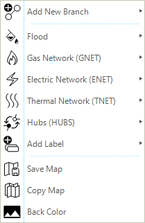
The user can access the background context menu of the map view by right-clicking on any map area with no network objects or objects selected. Figure 13 shows the background context menu for a map view where a gas, and electric, and a thermal network are loaded at the same time without scenarios.

The exact content of the context menu depends on the type of network, type of map view, and solved scenario active. Table 1 provides an overview of the main options.

Table 1. Context menu options for network types and scenario mode.
Options	Network mode	Scenario mode
Add new branch	Adds new (network) branch	-
Flood	Floods the subs, zones, groups, isolated areas, or hydraulic areas.	Floods the subs, zones, groups, isolated areas, or hydraulic areas.
Gas network (GNET)	Opens the gas network editor and remove redundant vertices.	Opens the gas network editor, remove redundant vertices, create a new plot in a plot window, or create network-level events and profiles.
Electric network (ENET)	Opens the electric network editor, remove redundant vertices, fuel, hydro plant, or ancillary service to the network.	Opens the gas network editor, remove redundant vertices, create a new plot in a plot window, or create network-level events and profiles.
Thermal network (TNET)	Opens the thermal network editor and remove redundant vertices.	Opens the gas network editor, remove redundant vertices, create a new plot in a plot window, or create network-level events and profiles.
Add Label	Add a new object or project label.	Add a new object or project label.
Save map	Saves the current map to a *.png file.	Saves the current map to a *.png file.
Copy map	Copies the map in its current state as an image.	Copies the map in its current state as an image.
Back color	Opens the color dialog window to change the color of the background of the map view.	Opens the color dialog window to change the color of the background of the map view.

4.1.5. Status bar

The status bar of the map view aims at informing the user, much like the project status bar, and shows some relevant information concerning the map view and the mouse location.

Figure 14 shows two examples of the status bar for a Cartesian map view (top) and a geographic map view (bottom) where it is possible to see:

the coordinates of the position of the mouse either as X/Y planar values or Lat/Long geographic values.
the service provider of the base map displayed in a geographic map view (the default is OpenStreetMap).
the default coordinate reference system used by the base map. The only accepted value is EPSG code 4326.
the number of selected nodes and branches.
the name of a selected object or the object the mouse if hovering on.
the slide bar for adjusting the mesh size of the grid lines, if the grid line option from the "Map Display Window" is turned on.
the zoom level of the active map view.

Figure 14. Examples of status bars for a Cartesian map view (top) and a geographic map view (bottom).

4.2. Map display settings

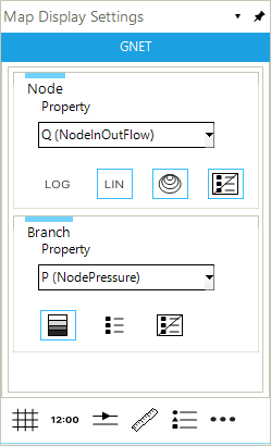
The "Map Display Settings" is the component of the map window controlling how network properties and results are visualized at the node or branch level. The user can specify the property of interest and define how the legend looks based on the personalization of colors, class intervals, type of scale (i.e., linear or logarithmic), size, and position in the map view. Figure 15 shows an example of the map display settings for a gas network where the calculated pressure at the nodes of a gas network uses a linear scale and a range defined by the global maximum and minimum. Branches describe the changes in the node inflow and outflow using the global maximum and minimum. The flow direction may be indicated by an arrow (i.e., third icon from left at the bottom).

Figure 15. Example of the "Map Display Settings" window for a gas network and an active solved scenario.

A blue box around an icon or a blue background indicates that the option is selected or turned on.

The "Branch" and the "Node" sections of the map display settings window are available when at least one network is active in current project. When multiple networks are loaded, a tab for each network type is available in the map display settings window. The properties in the drop-down list under "Node" and "Branch" differ based on the network and on the loaded solution.

The branch section provides three options:

Show the global maximum and minimum in the branch legend: icon : The option fixes the use of the global maximum and minimum from the entire network for the selected property. Alternatively, the extremes are calculated based on the values of only the displayed branches. By selecting this feature, the branch legend values will not change based on the values of the selected zoomed area.
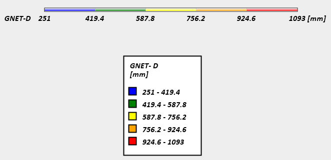
Switch to a single symbol in the branch legend: icon : The option switches between a bar legend and a patch legend for each class defined in the minimum and maximum numerical interval for the selected property (Figure 16).
Hide the branch legend: icon : The option removes any type of active legend and displays all branches using the default network symbology (i.e., lines with black segments and all other facilities with the their reference symbol).

Figure 16. Example of a bar legend (top) and of a patch legend (bottom) for a gas network describing the inner diameter of the pipelines.

The node section provides four options:

Logarithmic scaling of the node legend: icon : The scale used to represent values is set to a logarithmic scale with base 10.
Linear scaling of the node legend: icon : The scale used to represent values is set to a linear scale between the minimum and the maximum of the nodes displayed in the map window or the global extremes in the entire network.
Show the global maximum and minimum in the node legend: icon : The option fixes the use of the global maximum and minimum from the entire network for the selected property. Alternatively, the extremes are calculated based on the values of only the displayed nodes. By selecting this feature, the node legend values will not change based on the values of the selected zoomed area.
Hide the node legend: icon : The option removes any type of active legend and displays all nodes using the default network symbology (i.e., white dots with color-coded stroke).

The node section of the map display settings changes the fill color and the size of the nodes, but not the stroke color (i.e., the border color). The stroke color is fixed and uses the convention of "green" for a node with only external injecting energy in the system, "red" for a node with only external extracting energy from the system, and "orange" when both types of external are present. The stroke width and teh default node size can be changed from the context menu of the entry "Nodes" of the "Layers Window".

Branch and node legends display the default properties on the first load, and the user defaults (i.e., the user’s last selected properties) after. This applies to both network and scenario, and defaults are different for each scenario type.

The "map display settings" window exposes six more functionalities that control the other objects in the map view. In particular, we have:

Turn on/off the grid lines: icon : It turns the grid lines on/off in the map view to support the visualization. The spacing of the grid lines can be adjusted using a slide bar that appears next to the zoom level in the bottom-right corner of the map window. By default this option is off in a new project. Its status can be saved in a session for future use.
Turn on/off the time stamp: icon : It turns the time stamp for the active scenario on/off. In steady state cases is the start time of the simulation. In (quasi-)dynamic cases, it is the time stamp of the active step. By default this option is on when a scenario is loaded. Its status can be saved in a session for future use.
Turn on/off the line arrows: icon : It turns the arrows on/off on the branches indicating either the "from node - to node" construction direction or the direction of the scenario flow-related result. By default this option is off in a new project and when a network is loaded. Its status can be saved in a session for future use.
Turn on/off the scale bar: icon : It turns the visibility of the scale bar in the map view on/off. By default this option is on in a new project and when a network is loaded. Its status can be saved in a session for future use.
Turn on/off the network legend settings: icon : It turns on/off all active legends, overriding the nodes and branches options. By default this option is on in a new project and when a network is loaded. Its status can be saved in a session for future use.
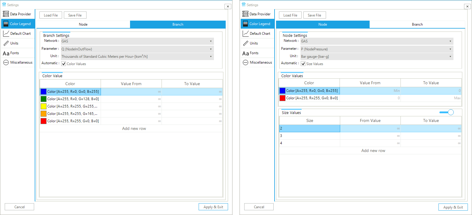
Open the map legend settings: icon : It opens the "general settings" section for the branch or node legend. Figure 17 shows the branch (left) and the node (right) tab of the general settings where the user can define the network, parameter, and unit of measure of interest.

From the tab "Branch", the user can:

select to automatically assign class intervals and colors to represent the parameter (i.e., tick the option "Automatic" for color values);
add new intervals to better divide the range minimum - maximum of the parameter;
change the color of any of the classes to better indicate a property;
manually specify the "Value From" and "To Value" for each class. The option "Automatic" must be unchecked. The "Value From" of the first class and the "To Value" or the last class are fixed to the absolute minimum and maximum respectively.

From the tab "Node", the user can:

select to automatically assign size intervals and change colors to represent the parameter (i.e., tick the option "Automatic" for size values);
decide to specify the size of the symbol, the number of size classes, and the range for each size with the "From Value"and "To Value" options. The "Value From" of the first class and the "To Value" or the last class are fixed to the absolute minimum and maximum respectively. The slide bar in the sub-window for size classes must be set to the right;
add new size classes to better divide the range minimum - maximum of the parameter. The slide bar in the sub-window for size classes must be set to the right.;
change the color of the classes to better indicate the positive and negative values of the selected property.

Figure 17. Example of the general settings for the branch legend (left) and for the nodes legend (right) accessible from the button

of the map display settings window.

Options in the map display settings are selected when either the icon has a blue border or a blue background (see the example of Figure 15)

The node legend can show only three different colors indicating the positive, negative or null values. The use can chose color options for negative and positive values. Null values are always in white.

The position of the legends in the map view is locked to the map view. Dragging or zooming does not affect the legend position.

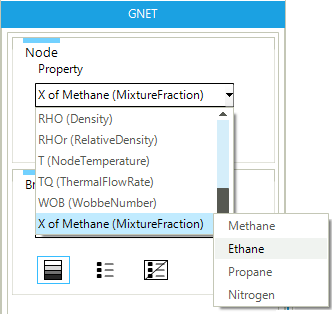
When selecting a certain property in the node or the branch legend, SAInt automatically calculates a valid legend, with default colors, and displays the results. One exception to this rule is when the user is interested in displaying the molar percentage or the mixture fraction of a certain quality component in a gas simulation. In this case, the user is required to select the specific component to visualize from a list accessible after clicking on the entry in the legend. See Figure 18 for an example.

Figure 18. To display the mixture fraction in the node or branch legend the use must select the component of interest by clicking on the entry "X of xxxx (MixtureFraction)". SAInt will provide a list to choose from and display the name of the component in the legend.

4.3. Layers window

Graphical objects, like labels, or modeling objects, like nodes, are displayed on a map view using layers, similar to raster or vector image editing software. A layer groups objects of the same type and provides a single entry point to common graphical properties.

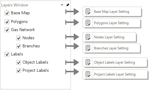
Layers are accessible from the Layers Window and depend on the type of map window (i.e., Cartesian or geographic), the number of networks loaded, and the availability of polygons and labels. Figure 19 (left) shows an example of a layers window for a geographic map view with one gas network (with its node and branches), a base map, polygons, and both object and background labels.

From the layers window, the user can quickly turn on/off the layer global visibility or, by right-clicking, access the context menu (Figure 19, right) of the layer and modify relevant graphical properties of the set of objects. The available context menus are:

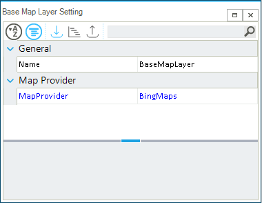
Base Map Layer Settings: the user can modify the map provider (MapProvider) used for the base map. A valid key for the map provider’s API must be specified in the "Miscellaneous" section of the general settings of SAInt. The setting specified for each map view can be saved and later restored from a saved session.
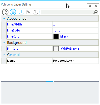
Polygons Layer Setting: the user can modify the appearance of polygons by specifying the line style (LineStyle), the stroke width (StrokeWidth) and the color (LineColor) of the boundary, as well as the fill color (FillColor) of the polygons (Figure 21).
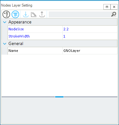
Nodes Layer Setting: for each network in the map window, the user can modify the appearance of the network’s nodes by specifying the size of the node symbol (NodeSize) and its stroke width (StrokeWidth) (Figure 22). The border color of a node is conventionally pre-defined in green (only supply externals at the node), red (only demand externals), and orange (both demand and supply externals). Refer to the section Map display settings for personalizing nodes when a solved scenario is available.
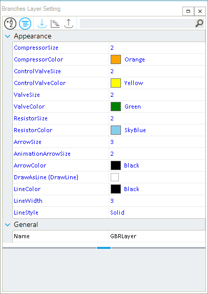
Branches Layer Setting: for each network in the map window, the user can modify the appearance of the network’s branches by specifying the size and color of the branch symbol (which depends on the type of network), the line width (LineWidth) and style (LineStyle) of pipelines and electric lines, and the color and size of the arrow symbol used in the map view or in an animation (ArrowSize, AnimationArrowSize, ArrowColor) (Figure 23).
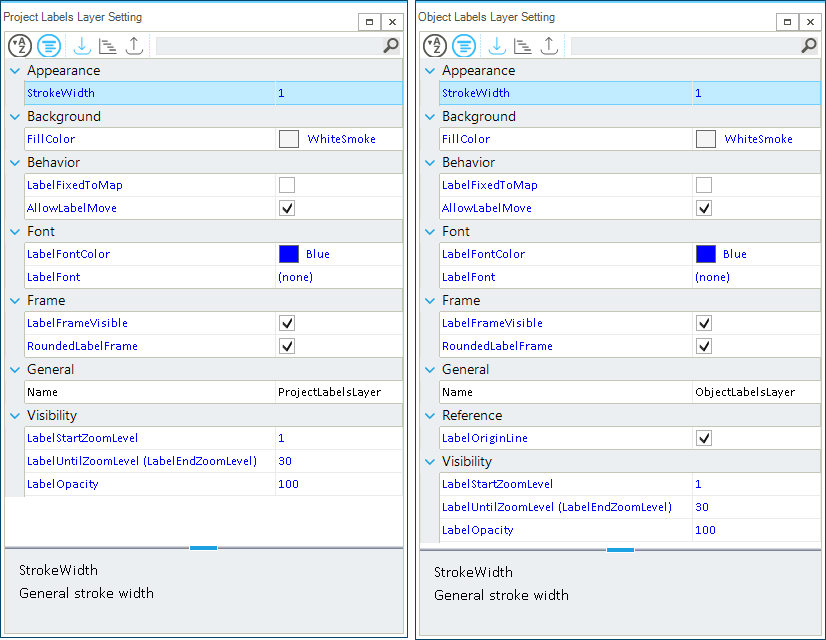
Project Labels Layer Setting: the user can control the graphical properties and placement behavior of project labels by changing border and fill color, transparency, font attributes, framework type, and size, and zoom range (Figure 24, left).
Object Labels Layer Setting: the user has the same level of control for object labels as for project labels. With the exception of the callout (LabelOriginLine), project and object labels share the same properties (Figure 24, right). For more details refer to the section Labels and label properties. For more details, refer to the section Labels and label properties.

Finally, it is possible to use the layers window to quickly re-center the map view to display the full extent of one of the loaded networks. Just double-click with the right mouse button on the entry "Gas Network", "Electric Network", or "Thermal Network" to center the map view to that network. On the other hand, by clicking with the mouse wheel in the map view, the extent is refresh to show all loaded networks.

Figure 19. Example of the "Layers Window" with one gas network, a base map, polygons, and object and background labels. On the right, the context menu accessible by right-clicking on the entry on the left.

Figure 20. Settings of the graphical properties of the base map layer from the context menu of the layers window.

Figure 21. Settings of the graphical properties of the polygons layer from the context menu of the layers window.

Figure 22. Settings of the graphical properties of the nodes layer from the context menu of the layers window.

Figure 23. Settings of the graphical properties of the branches layer from the context menu of the layers window for an example of a gas network. For other types of networks, the list of available objects under the Appearance section is different.

Figure 24. Settings of the graphical properties of the object labels (left) and project labels (right) from the context menu of the layers window.

User-specified object-level graphical settings have higher priority than user-specified layer-level graphical settings. For example, changing the size of nodes from the layers window affects all nodes, apart from the ones where the size is already specified using the node property editor (i.e., at the object level).

Polygons are available on Cartesian map views only. With future releases polygons will be supported in geographic map views as well.

4.4. Node bar

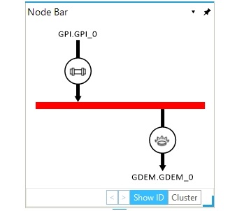
The node bar displays externals and branches connected to the selected node. The user can choose different display options of the node bar using the Show Id and Cluster located on the bottom right of the node bar window. The first option labels each element in the node bar with its full identifier. The second option groups objects of the same type together and labels them by type if "Show ID" is also active. An example is shown in Figure 25. The Node bar window is generally located on the right side of the map window. By default is docked. The other editable property of the node bar is its background color. Open the context menu by right-clicking on any empty area of the window.

The color of the main horizontal line follows the rule: red if the node has only demand externals linked, green for only supplying externals, and orange for a mixed situation.

Each element connected to a node is also associated with an arrow. The direction of an arrow in the node bar indicates:

All Networks

Demand: Outwards directional arrow.
Branches: Depends on the defined FromNode and ToNode of the branch.

Gas and Electric Networks

Storages: Bi-directional arrow.

Gas and Thermal Networks

Supply: Inwards directional arrow

Electric Networks

Generator: Inwards directional arrow.
Shunt: Outwards directional arrow.

The user can choose different display options for the node bar using the ShowId and Cluster located on the bottom right of the node bar window.

Figure 25. Example of a "Node bar" window in "Show ID" mode where the gas node is connected to only one pipeline and to a demand external.

4.5. Map selection filter

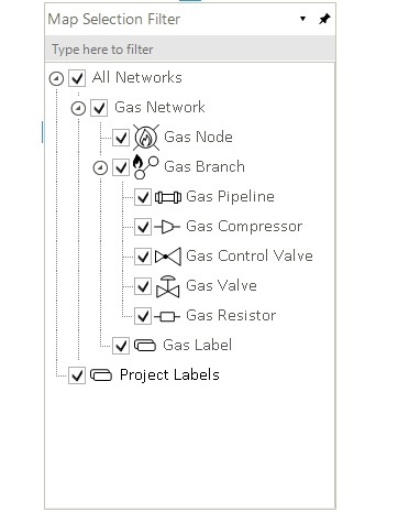
The map selection filter is shown in Figure 26. It is used for filtering the selection of network objects in the map window using the shift key and holding the left mouse button.

When an entry is unchecked from the selection filter, all the associated objects will not be selectable any more in the map window.

Figure 26. Example of the "Map selection filter" window for the case of a gas network.

4.6. Labels and label properties

Labels are a flexible tool to display properties or results for a specific object (i.e., an "object label" or a "network label") or to add text and information to a map window (i.e., a "project label"). The user can simply add a label to an object from the context menu with Add New Object Label To after selecting the object. Or add a network or project label to a map view using the context menu after right-clicking in any area of the view away from objects.

A "project label" only accepts free text. Compared to object or network labels, the syntax used for extracting and displaying properties or results is not interpreted but is considered as a normal string. Furthermore, a project label is not linked to any network, so it is displayed even when there is no network at all. For this reason, project labels are great for having informative text describing your project.

For more details, check the How-to guides "Add Labels" and "Edit Labels".

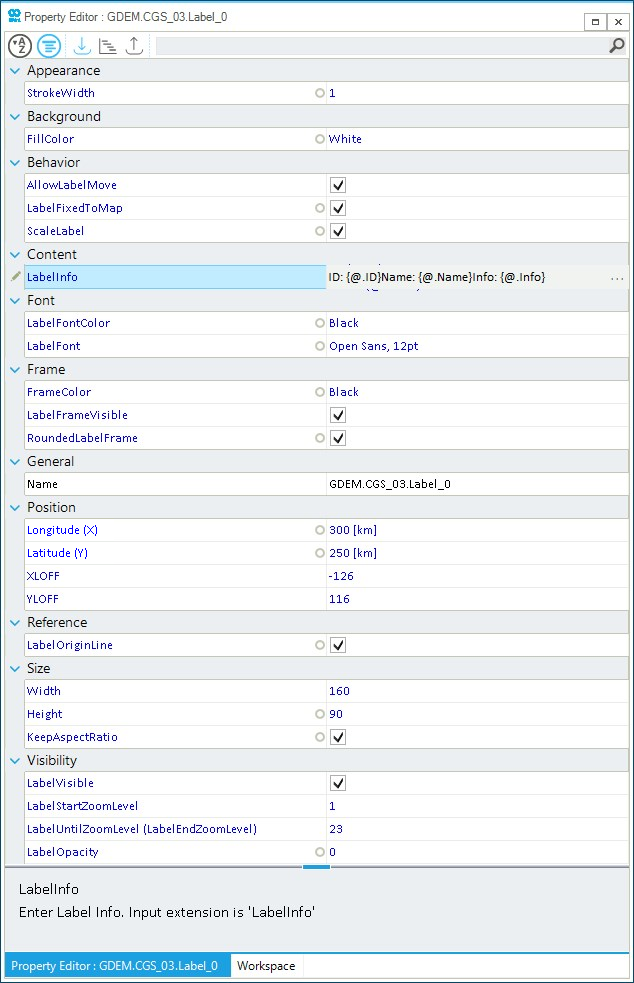
Once a label is added, it is possible to personalize its content and graphical appearance through the property editor. The user can access the property editor for a label either by selecting the label if a property editor was already open or by right-clicking on the label and from the context menu select Open Editor. Figure 27 shows an example of the property editor for a label linked to a GDEM object. The user can modify:

the appearance of the frame around the label by setting the stroke width (StokeWidth under Appearance);
the fill color of the label frame (FillColor under Background);
the color and visibility of the label frame, along with the type of corners (i.e., round or sharpe)(FrameColor, LabelFrameVisible, and RoundLabelFrame under Content);
the size of the frame for height, width, and aspect ratio (Width, Height, and KeepAspectRatio under Size);
if the frame has a callout to the object linked to the label (LabelOriginLine under Reference);
the visibility of the label can be turned off or on, as well as the transparency of the label or the zoom range for which the label is drawn can be changed (LabelVisible, LabelStartZoomLevel, LabelEndZoomLevel, and LabelOpacity under Visibility);
the label position either based on the map view coordinates or relative to the position of the linked object with screen coordinates (X, Y, XLOFF, and YLOFF under Position);
if a label is at a fixed position or can be moved around the map window if the position is based on map coordinates (the X and Y of the section Position) or as offset from the linked object (the XLOFF and YLOFF), and if the label size must be rescaled based on the zoom level or fixed to a specific size (AllowLabelMove, LabelFixedToMap, and ScaleLabel under Behavior).

For a detailed description of the property editor, refer to Section 6.

The visibility of a specific label is controlled by its property LabelVisible. The visibility of all labels in a map window is controlled from the "Layers Window".

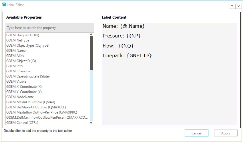
The transparency of the background is controlled either by LabelOpacity under Visibility or by FillColor under Background. LabelOpacity accepts values between 0 and 100. The tab "Professional" in the "Color dialog" accepts values between 0 and 255 for "A". The two values are linked and remapped in the corresponding intervals

The LabelInfo property under Content allows the user to modify the default content of any label. By clicking on the three dots next to the string content of the LabelInfo property, the Label Editor opens (Figure 28). In the label editor, the user can mix free text with tags for the object’s properties and results of simulations. On the left side, a filtrable list is available with all properties and results for the object type the label is linked to. On the right side, the user can compose the content of the label using a simple syntax. Properties or results are indicated by {@.PROPERTY} where the object is either explicitly mentioned or implicitly referred to using @ (i.e., the same object linked to the label). A property is indicated using the property symbol in SAInt. It is possible to indicate the unit of measurement for the selected property even if different from the one specified in the general settings of SAInt. The syntax of the tag requires that the fields used are separated by a dot and within curly brackets as in {@.XXX.YYY.[xxx]}. In the example of Figure 28, the label for this GDEM object will show the name of the demand external, its pressure, the outflow, and the network linepack on four different lines. All numeric values use the project settings units of measurement and are valid for the active simulation time step or network state.

For details on how to use the label editor and examples of label syntax, refer to the How-To guide Edit Labels.

Figure 27. Example of the personalization properties a user can modify from the property editor for a label linked to a GDEM object.

Figure 28. Example of the label editor for a GDEM object showing the name of the external, the pressure, the outflow, and the network’s linepack for the active time step - or network status - and using the project’s settings units of measurement.

Label properties defined in the context menu accessible from the Layers Window have lower priority over the properties defined at single label level.

The "Copy&Paste" options works for branches and nodes directly in the map view. For externals, the options work in the model explorer. Project labels do not have such options.

5. Script editor

The script editor is accessible from the tab "View" and the menu entry Script. The user can either create a new script using the option Create New IronPython Script or load an existing script using Open Ironpython Script. The script editor allows the user to create and save customized codes using IronPython functionalities. Similar to the command window, it uses the IntelliSense feature to guide the user in entering the commands. Lines are numbered for convenience, and different colors are used to help the user to navigate the code and quickly recognize the type of command used. An example of using the script editor is shown in Figure 29.

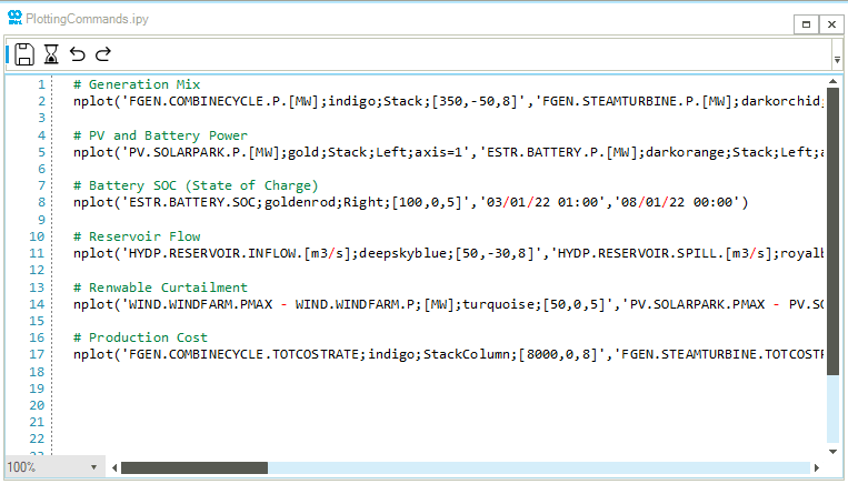
Figure 29. Example of the use of the "Script Editor" with an IronPython script named "PlottingCommands.ipy" for user-defined nplot commands.

In the top section of the script editor window, four customizable buttons are available for a quick access to the following options:

Execute script: Executes the current script. SAInt objects referred in the code are accessed based on either the active time step or the solved solution for the active scenario.
Save script: Saves the current script with *.ipy extension.
Undo changes: Undo the recent changes in the script.
Redo changes: Redo the recent changes in the script.

Buttons can be customized using the context menu at the right side of the buttons bar.

The user can also change the zoom level of the text of the script editor by pressing CTRL and using the wheel of the mouse.

Errors or exceptions caused by the execution of IronPython scripts are reported by SAInt using a pop-up window.

You can start learning more on expressions and functions by looking at the section "Functions, Expressions and Conditions" of the reference guide.

6. Property editor

The property editor is accessible from the window "Property Editor" located on the right-most window of the SAInt-GUI or from the tab "View" and the menu entry Script in the tab "View". The property editor allows the user to edit all types of properties of a network’s object or a scenario’s event. The editor filters the list of properties depending on the type of selected object or loaded scenario.

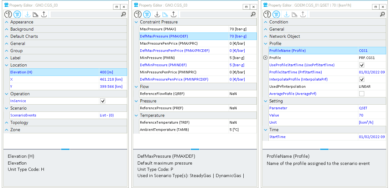
Figure 30 shows examples of the property editor window when an object (left, center) or a scenario event are selected (right). The figure shows how the property editor window is divided into three areas: the toolbar at the top, the "table" section in the middle, and the "information box" at the bottom.

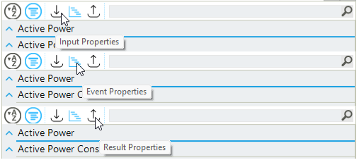
Figure 30. Examples of the "Property Editor" window when the "input property" section for an object is selected (left; in this case is the gas node GNO.CGS_03), or the "event properties" section is selected (center), or when the "input property" section for a scenario event is active (right). In all cases, the window is dived into toolbar (top part), table section (central part), and information box (bottom part).

The toolbar has two buttons (i.e., first two icons on the left), three tabs and a search bar, as shown in Figure 31. By hovering the pointer over the tabs a description is displayed. The available options are:

Sort alphabetically button: Sorts the properties alphabetically (A-Z or Z-A).
List button: Sorts the properties by category.
Input tab: Shows the input properties, which are properties related to the network object.
Event tab: Shows the event properties, which are properties related to the specified event.
Results tab: Shows the result properties corresponding to the loaded scenario.
Search bar: Searches for a specific property.

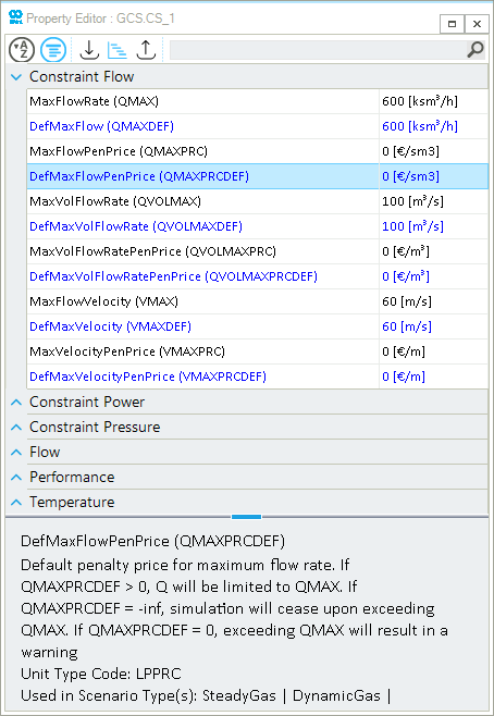
The "table" section of the property editor has two columns. The left column has the property names, while the right column has the corresponding property values (Figure 32).

The user can modify any property in blue by double-clicking on the property value or using the Edit option from the context menu. The following options are available in the context menu:

Reset: Resets the property value to default or previous value.
Edit: Edits the property.
Expand: This option is only active when a property contains a list.
Sort: Sorts the properties alphabetically, by category, and alphabetically categorized. Selecting this option changes the entire property editor.
Show description: Controls the visibility (ON or OFF) of the description bar.
Show toolbar: Controls the visibility (ON or OFF) of the toolbar.
Copy expression: Copies the property expression.

The left side of the value cell shows three different types of symbols, depending on the property type, when the user clicks to modify the cell’s value. One option is to have a triangle-shaped symbol, which indicates the presence of a drop-down menu to select a possible value from a validated list. When a numeric field is selected, a second option is available. Next to the numeric area the user has the indication of the unit of measure, optionally the symbols for plus and minus infinite, and small triangle-shaped buttons to increase or decrease the numerical value. The third option is to have a small triangle-shaped symbol inside a circle next to the name of the property (i.e., on the left side of the cell value field), by clicking on the symbol the cells unfolds revealing a nested hierarchy of child properties. A good example is under "Topology" the entry "Points" for an electric line or a pipeline object.

The user can only edit the properties with blue color. The non-editable properties are in black.

Figure 32. Example of the "Table" section (top) and "Information box" section (bottom) of the property window.

The property editor for different object types can be accessed in a variety of ways in SAInt-GUI:

Objects: The property editor for each network object (e.g., EDEM, TNET, GNO, EDGCS) is available from the context menu after selection of the object either in the map window, the model explorer, or the node bar. Just choose the entry Open Editor.
Scenarios: The property editor for a scenario event (e.g., PSET, VOLSET, FuelPrice, etc.) is accessible from:
- Scenario Tab: by selecting an event in the scenario table under the Scenario tab and button GSCE for a gas scenario, ESCE for an electric scenario, or TSCE for a thermal scenario.
- Project Explorer: Selecting the scenario from the entry Scenario Files in the project explorer and using the open editor option from the context menu.
Network editor: The property editor for a network is accessible from the following locations:
- Network tab: Clicking on the button GNET, ENET, TNET or HUBS, for a gas, and electric, a thermal or a hub system respectively, under the Network tab in the ribbon bar
- Map window: Using the entry Gas Network (GNET) Open Gas Network Editor, Electric Network (ENET) Open Electric Network Editor, Thermal Network (TNET) Open Thermal Network Editor, or Hubs (HUBS) Open Hubs Editor from the context menu of the Map Window. To access these context menu options, no network objects should be selected.
- Model explorer: Selecting a network and using the entry Open Editor from the context menu of the network object.
- Project explorer: Selecting the network from network files and using the entry Open Editor option from the context menu of the network.
Profile editor: The property editor for a profile is accessible from the following locations:
- Model explorer: Selecting the profile from the entry Profiles and using the Open Editor option from the context menu of the profile.
- Profile table: Using the entry Open Editor from the context menu of the profiles shown in the profile table. The profile table is accessible from the button EPRF for electric scenarios, GPRF for gas scenarios, or btn:TPRF[] for thermal scenarios, under the Scenario tab.
Events editor: The property editor for the events is accessible from the following locations:
- Model explorer: Selecting the event from the entry under Scenario Events and using Open Editor option from the context menu of the event.
- Event table: Using the Open Editor option from the context menu of the events shown in the event table. The event table is accessible from EEVT for electric scenarios, GEVT for gas scenarios, and TSCE for thermal scenarios under the scenario tab.
Polygon editor: The property editor for the polygon is accessible from the following locations:
- Model explorer: Selecting the polygon file under the entry Polygons and using Open Editor from the context menu.
- Polygon table: Using the Open Editor option from the context menu of the polygons shown in the polygon table. The polygon table is accessible from PLG under the table tab.
Label editor: The property editor for a label is accessible from the map window, after selecting the label, by choosing the entry Open Editor of the context menu.

If the property editor is open, its content will adapt automatically to the object selected by the user.

The user can interact with multiple objects of the same type in a multi-edit session of the property editor. Simply select the set of objects of the same type either in the map window or the model explorer and from the context menu choose Multi Edit. The title bar of the property editor will report the number of objects selected.

The list of properties is filtered so that the editable ones are available. If an entry is empty, the selected objects have different values for the field. When the value is the same among all objects, it is available in the multi-edit window.

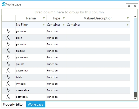
7. Workspace

The workspace is accessible from the tab "Workspace" located on the right-most window of the SAInt-GUI. It is in auto-hide mode by default. It lists the predefined functions used in the command window and script editor of SAInt. The list includes the name, syntax, and the description of the functions. A snapshot of the part of workspace is shown in Figure 33. It consists of three columns:

First column: Name of the function or command.
Second column: Type of the command. This column is related to the icon used on the row for the entry. Where, for example, a "function" type uses an icon with "f_X", or a Boolean type uses two intersecting circles. Other types are: string, list, or float.
Third column: Description of the function.

The user can interact with the workspace window by:

Sorting: The columns can be sorted alphabetically by clicking on the column headers.
Filtering: The filtering options for the columns can be accessed by clicking the filter icon next to the column name.
Moving: The columns location can be changed by dragging the column to the desired location.
Grouping: The columns can be grouped by Name, Type, and Value/Description by dragging the column header to the top of the workspace table in the row that says ""Drag column here to group by this column.
Search: The search bar is available in the filtering options (filter icon next to the title) for each column.

You can start learning more on expressions and functions by looking at the section "Functions, Expressions and Conditions" of the reference guide.

Figure 33. Example of a subset of functions from the "Workspace Window".

8. Command window

The command window is located on the bottom-left below the map window by default. It is a platform that uses pre-defined functions in an IronPython environment to perform various tasks such as mark objects, create plots, tables, or evaluate properties. It uses IntelliSense features to guide the user in entering commands. An example of using the command window is shown in Figure 34.

You can start learning more on expressions and functions by looking at the section "Functions, Expressions and Conditions" of the reference guide.

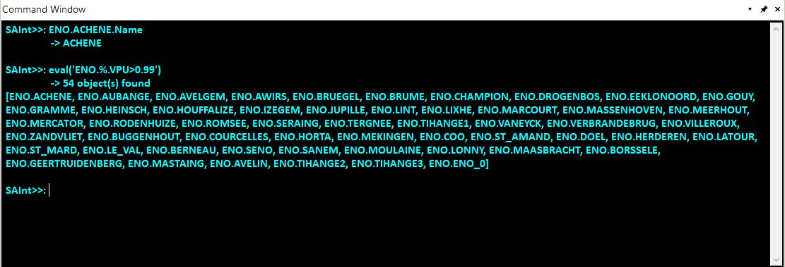
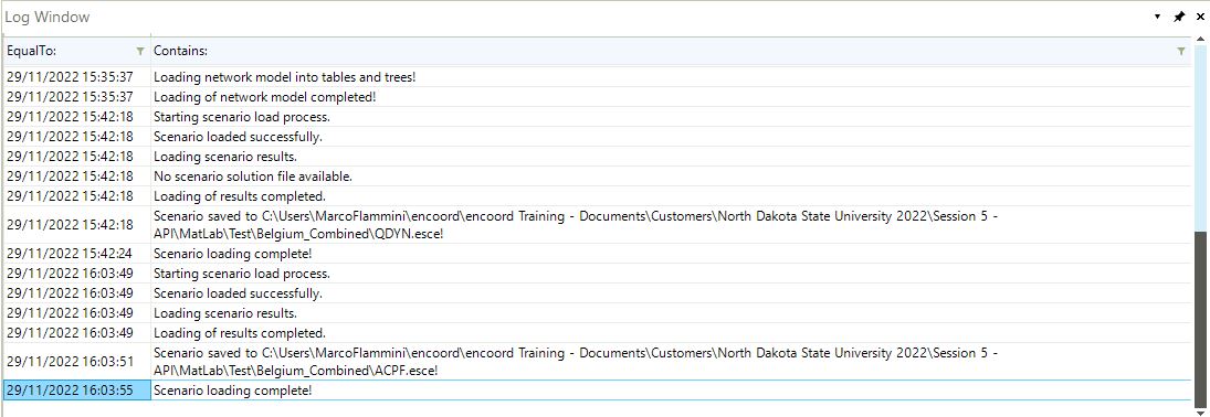
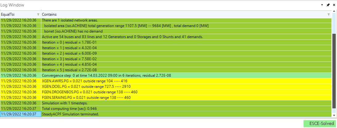
Figure 34. Example of the use of the "Command window" to retrieve the property Name of an electric node or to evaluate an expression where the condition VPU>0.99 is satisfied.

9. Log window

The log window is by default in the bottom-right area below the map window. It is the primary source of information for SAInt-GUI operations. It shows the log for network and scenario operations including the simulation or optimization logs. Figure 35 and Figure 36 shows the snapshot of the log window showing the operation and simulation logs, respectively. It has two columns with available filtering options such as contains, not contains, starts with, ends with, equal to.

The first column reports the start date and time of the operation/simulation. The time and date is based on the settings of the computer used to run SAInt.

The second column reports the message from the SAInt solver or GUI for the specific action taking place. Colors are used in simulation or optimization logs to indicate warnings (yellow) or errors (red). Other informative messages use shades of green.

Figure 35. Example of the "Log Window" with operation logs.

Figure 36. Example of the "Log Window" with simulation logs.

Only simulation logs are displayed once the user starts the simulation.
The user can check or uncheck the AutoScrolltoBottom property of the log window under the Application Menu Settings Miscellaneous Tab. It locks or unlocks the scroll vertical bar of the log window at the user-defined position when new rows with logging information are being added.

10. Chart window

The "Chart Window" is a component of the dock panel specialized in interactively plotting charts. The user can always generate a chart in its own window by using the context menu of an object or event or by using the plot or nplot commands in the command window.

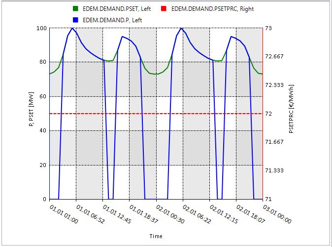
The chart window is accessible from the tab View in the ribbon bar and the menu Chart. It displays plots for one or multiple network object properties or events. The plots can either be derived from the results of a simulation/optimization, from input parameters, or from an event. An example of a plot illustrating active power set point (PSET), active power (P), and penalty price for demand curtailment (PSETPRC) over a period of two days is shown in Figure 37.

For detailed information on the plotting commands, refer to the section "Plot Functions" of the reference guide.

For more details on how to build expressions to be plotted, refer to the section "Functions, Expressions and Conditions" of the reference guide.

Figure 37. Example of a chart in the "Chart Window".

The user can create and visualize plots in multiple ways:

by using any valid plotting command for charting properties and results.
by using the entry Plot Window and choosing a specific chart from the context menu of any object selected either from the model explorer, the map view, or the node bar.
by using the entry Plot Event or Plot Window from the context menu of a selected event in the event table of the active scenario.
by having a "chart window" open and selecting an event or an object

All the options, with the exception of the first, require an active and solved scenario. With option from one to three, the chart is generated in its own chart window. With option 4, the same chart window is used and updated for any new selected object or event.

The user can interact with the chart window in four ways:

Zooming in/out by using the mouse wheel. Chart axis are re-scaled according to the zoom area. SAInt does not offer a drag-and-zoom feature, but the user can easily zoom at the position of the cursor.
Reset the default zoom level by clicking on the mouse wheel button.
Navigate through the zoomed plot using the mouse wheel and pointer (when the option "Lock Vertical Zoom" is unchecked in the context menu).
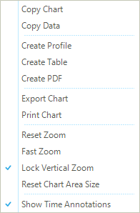
Using the context menu of the plot (Figure 38)
1. Copy Chart: to copy the chart for pasting into another document.
2. Copy Data: to copy the time steps and the corresponding values of the chart for pasting into an Excel or Notepad file.
3. Create Profile: to create a profile from the values of the chart. The name of the profile follows the name of the object and acronym PRF.
4. Create Table: to create a table with the time series data of the chart.
5. Create PDF: to save the time steps and the corresponding values of the chart to a table in PDF format.
6. Export Chart: to save the chart to an image file.
7. Print Chart: to open a print preview window.
8. Reset Zoom: to reset to the default zoom level.
9. Fast Zoom: to activate an automatic "zoom in" operation based on the mouse pointer’s position and the optional locking on the vertical axis.
10. Lock Vertical Zoom: to lock the zooming so that the vertical axis is fixed and only the horizontal is changed.
11. Reset Chart Area Size: To reset each plot to have the same area in a subplot chart.
12. Show Time Annotation: To toggle on or off the use of the time annotations in event plots.

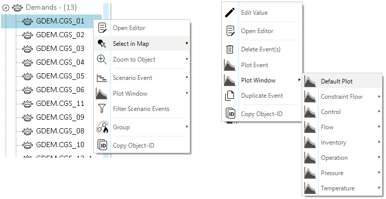
SAInt has two types of charts: plots for an object’s properties and plots for events associated with it. From an entity’s context menu, it is possible to clearly choose between "Plot Window" for the first type and "Plot Event" for the second type. See Figure 39 for an example.

In the "Plot Window" class, SAInt provides the user with the option of creating and personalizing a "Default Plot" for the selected object. Default plots can be changed by modifying the linked plotting command from the general "Settings" ("Default chart"). The user can change any default chart with a new one, or modify the colors, the legend and title, or the type of chart for a specific property. The default charts can be saved to an external file and restored from an external file.

The "Event Plot" class is available only for events. Depending on the type of network and the type of event, the event chart has a specific graphical output. In an event plot the user can see all or some of the following elements (Figure 40 and Figure 41):

time annotations with some vertical text, which can be toggled on or off from the chart context menu. There are different types of annotations:
- the scenario start time indicated by a vertical annotation stating "ScenarioStartTime" followed by the date and time.
- a profile start and end time by vertical annotations stating "ProfileStartTime" and " ProfileEndTime" followed by the date and time. The user can see the actual time span of the original data of a profile.
- the event start time is indicated by a vertical annotation stating "EventStartTime" followed by the date and time of the event.
axis:
- the horizontal axis is always representing time.
- the left vertical axis describes either the control modes of the object associated with the event or the user-specified values for the event. When the control mode is plotted, the state of all events in the scenario for the same object is reported.
- the right vertical axis describes the event’s values (or the value multiplied by a profile) if the left vertical axis is describing the control modes.
graphical elements with a color-coded meaning:
- when present, a "green" line indicates the user-specified "value" for the event (or the value multiplied by a profile) in the time window defined by the "event start time" up to either the end of the scenario or to the next event for the object. The plotted values are not to be confused with the actual computed values by SAInt, as the two sets may be different because of constraints handling and penalty prices.
- a "blue" line indicates either the sequence of events associated to the object in the active scenario or the user-specified "value" for the event (or the value multiplied by a profile). The user-specified values are present only when the event has no control mode associated. Otherwise, the control mode is represented in blue, and the user-specified values in green. It is important to stress that the realized sequence of events or values during a simulation may be different from the planned in the scenario as constraint handling may occur.
- for gas events, a "purple" line over the blue line indicates the portion of the chart referring to the selected event. If an object is associated to multiple consecutive events, SAInt indicates the section of the chart for the selected event used for creating the chart with a purple overlapping line to the blue line.
- when present, a "pink" line indicates a user-defined default value linked to an object. This is useful for comparison. The default value is, generally, indicated with an axis on the right side of the chart.
- for electric events, when present, a "red" line indicates the evolution of the event value before the selected event start time.
graphical elements with a style-coded meaning:
- a continuous line indicates a sequence of (active or not) events or values as specified for a certain object in the active scenario. For example, a continuous line is expected to be used for green, blue or red lines.
- for gas events, a dashed line indicates the time window in a simulation defined by the start time and the first user-specified event in the active scenario. This line pattern indicates what is inherited from the initialization state. This is equivalent to the use of a red line in charts of electric events. We avoided to add the red color to gas event charts to reduce the total number of colors.

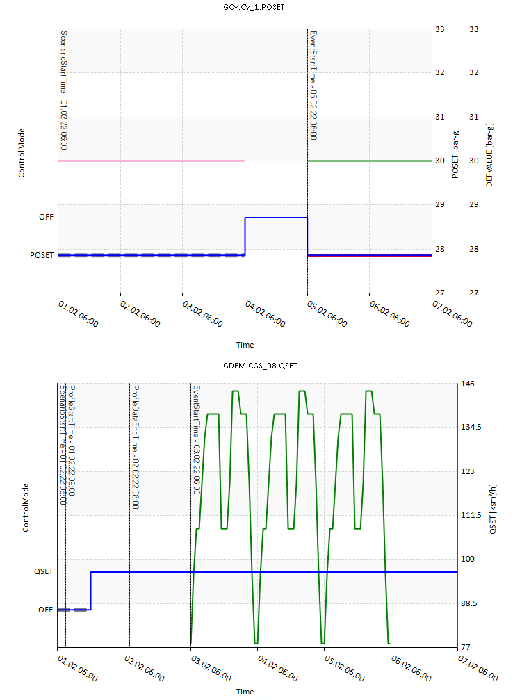
Figure 40. Example of "Plot Event" for a POSET event for a gas control valve GCV.CV_1 object (top) and for a QSET event with a profile for a gas demand GDEM.CGS_08 object (bottom). The graphical elements in the charts demonstrate the set of rules valid for an event chart.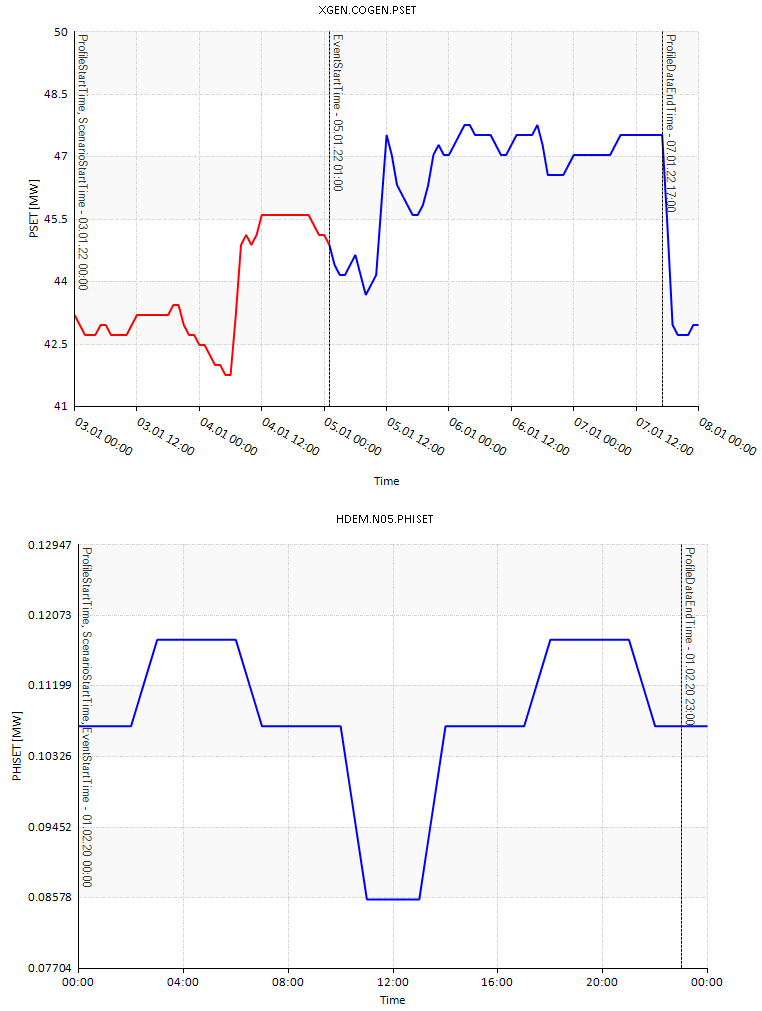

Figure 41. Example of "Plot Event" for a PSET event for an electric generic generator XGEN.COGEN object (top) and for a PHISET event with a profile for a thermal demand HDEM.N05 object (bottom). The graphical elements in the charts demonstrate the set of rules valid for an event chart.

Dock Panel

1. Window interaction and positioning

2. Project explorer

3. Model explorer

3.1. Context menu in the model explorer

4. Map window

4.1. Map view

4.1.1. Types of map view

4.1.2. Base map types

4.1.3. Content of a map view

4.1.4. Background context menu

4.1.5. Status bar

4.2. Map display settings

4.3. Layers window

4.4. Node bar

4.5. Map selection filter

4.6. Labels and label properties

5. Script editor

6. Property editor

7. Workspace

8. Command window

9. Log window

10. Chart window