Thermal Scenarios
A thermal scenario describes the operation of a gas network according to conditions specified in scenario properties and events. The conditions at which these variables are evaluated are specified by the events and profiles of the thermal scenario. The properties and settings of a thermal scenario define its time span and resolution, as well as the mathematical equations (e.g., equation of state) and numerical tolerances adopted for the solution. The types of thermal scenarios that can be selected in SAInt are "steady state scenario" (SteadyThermal) and "quasi-dynamic scenario" (QuasiDynamicThermal).
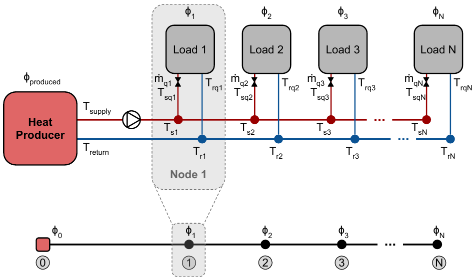
A thermal network delivers heat from supplies to demands based on the transportation of working fluid (liquid, non-compressible) and heat exchangers. The transportation of fluid must be described, and the equation is largely simplified compared to that for a compressible gas. Furthermore, the devices to be modelled are similar to those for a compressible gas. However, the heat transferred into/out of the working fluid is usually specified. That is, the event in the scenario is not related to flow but heat. Thus, another set of equations to describe the relationship between temperature and heat must be taken into consideration. There are two viewpoints in a thermal network, illustrated by the following image:
-
At the top, the hydraulic viewpoint sees the network being two parts, hot and cold. The water is pumped to circulate within pipes and heat exchangers.
-
At the bottom, the heat viewpoint focuses only on the hot part, which delivers heat from supplies to demands.
1. Steady state scenario
A steady state thermal scenario (SteadyThermal) is used to analyze a snapshot of the operation of a thermal network. It describes a condition for a thermal network where the parameters that characterize the heat flow and the network objects are independent of time (i.e., we assume that the system is in a state of equilibrium).
The properties of a SteadyThermal scenario allow specifying solver and time-related information, as well as general attributes and chart visualization options, when accessed using the property editor. Solver settings provide control over the residual tolerances and the maximum number of iterations admitted during the numerical solution of the steady state fluid-dynamic problem. Time settings are included too, being steady state scenarios conventionally assigned with a 1-hour time window and time resolution.
Table 1 provides an overview of the solver’s properties for a SteadyThermal scenario, while Table 2 shows the conventional "time-related" properties.
| Display name | Description |
|---|---|
|
The residual tolerance for linearization steps. The default is 1.0E-5. |
|
The maximum number of iteration steps for linearization. The default is 50 steps. |
| Display name | Description |
|---|---|
|
Start time of the scenario. The default is to set the calendar day and hour of when the scenario is created. The property is not relevant to the solution of a steady state simulation. |
|
End time of the scenario. The default is to set the calendar day and one hour plus of when the scenario is created. The property is not relevant to the solution of a steady state simulation. |
|
Total simulation time window. It is set to a fixed one-hour duration. The property is not relevant to the solution of a steady state simulation. |
|
Time step for the scenario. The property is fixed to 60 minutes, and it is not relevant for the solution of a steady state simulation. |
|
The number of time steps for the scenario time window. The property is fixed to 1 time step, and it is not relevant for the solution of the simulation. |
2. Quasi-dynamic scenario
A quasi-dynamic scenario allows for the assessment of the operation of a thermal network under "time-ordered" boundary conditions and network object properties. A quasi-dynamic thermal scenarios is a succession of independent steady simulations where events and conditions for each snapshot changes with time, but a single snapshot is evaluated under steady state conditions (i.e., assuming an equilibrium state). SAInt searches for a steady state converged solution at time step "tn", after a solution for time step "tn-1" has been found and checked for the absence of bound violations.
The properties of a quasi-dynamic scenario allow the user to specify solver settings, time-related information, general attributes, and chart visualization options when accessed using the property editor. Solver settings provide control over the residual tolerances and the maximum number of iterations admitted during the numerical solution of the quasi-dynamic thermal problem formulation. The time settings for a quasi-dynamic scenario define the simulation time window, the start time and the end time, the time step, and an optional scenario providing the initial conditions, constituting the operational snapshot of the system prior to the beginning of the scenario. Table 3 provides an overview of the solver’s properties for a quasi-dynamic scenario, while Table 4 shows the time-related properties.
| Display name | Description |
|---|---|
|
The residual tolerance for linearization steps. |
|
The maximum number of iteration steps for the problem linearization. |
| Display name | Description |
|---|---|
|
The start time of the scenario. This is the first time step in a scenario. The default is to set the calendar day and hour of when the scenario is created by the user. |
|
The end time of the scenario. This is the final time step in a scenario. The default is to set the hour and a plus one calendar day of when the scenario is created. |
|
The total simulation time window or the total amount of time in a scenario (i.e., the difference between |
|
A time step is a fraction of the scenario time window used for discretizing the scenario time window into distinct time points which are calculated for the variables. The time window is a multiple of the time step, i.e. |
|
The number of time steps for the scenario time window (i.e. |
|
Name of the scenario whose terminal state is used as the initial state for the current scenario. This is an optional property, and the default is set to none. The property is in the "General" section of the property editor. |
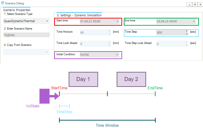
Figure 2 shows an example of the time settings and the associated graphical description of a quasi-dynamic thermal scenario as available in the Scenario Dialog window. The settings are for a scenario named "TQDYN" covering a 48-hour time window and using a time step of 15 minutes from April 4 at 00:00 to April 3 at 00:00. No initialization state is specified.
3. Stopping criterion
The stopping criterion decides when the simulation should stop iterating. The criterion is checking whether the intended numerical accuracy has been achieved by comparing the max absolute value of the residuals against the user-defined residual tolerance (i.e., ResidualTolerance). The iteration continues if the residual exceeds the tolerance and the maximum user-defined number of iterations (i.e., MaxIterationSteps) has not been exceeded.
Different types of equations are used to model the thermal network. Their physical quantities are different. For this reason the quantity ResidualTolerance is calculated using different units of measurement during its comparison with the residuals.
| Equation type | Object type | Unit of tolerance |
|---|---|---|
Pressure drop |
Thermal pipe |
kPa |
Heat balance |
Thermal node |
kW |
Temperature drop |
Thermal pipe |
K |
Temperature drop |
Thermal external |
kW |
For example, when ResidualTolerance is 0.01, in terms of the pressure drop equation, a converged solution indicates all the residuals are between -0.01 [kPa] and 0.01 [kPa].