Performing Time-Domain Reduction on CEM profiles
This section explains how to perform time-domain reduction to decrease the temporal resolution of a CEM dataset using pySAInt. The process can be approached in two ways:
-
Using Existing CEM: Start by editing the CEM previously generated, as detailed in the "Edit a CEM" section. Once the CEM is loaded, you can proceed with the time-domain reduction.
-
Creating a New CEM: Alternatively, if starting from scratch, create a new electric dataset. Populate it with the necessary CEM object properties, scenario details, horizon input, events, and profiles. After setting up the CEM, carry out the time-domain reduction.
Both methods provide flexibility depending on whether you are working with existing data or starting from scratch. In this guide, we will use the first approach and read the CEM input files generated from the "Build a CEM" section.
1. Initialize the pySAInt Dataset
import pysaint as ps

# This creates an empty electric dataset
dataset = ps.create_electric_dataset()
2. Read CEM Input Files
The read_cem_input_files method is designed to populate an existing pySAInt dataset with data from CEM input files. It accepts the following parameters:
| Parameter | Type | Description |
|---|---|---|
path_or_buf |
str |
Path to the CEM Input folder containing the CEM input files. |
cem_scenario |
str |
CEM scenario name, containing the input data from the CEM input files. |
|
Ensure to update the directory path to where the CEM input files are stored. The example below uses the path to the directory containing the CEM input files generated in the "Build a CEM" section. |
import os

# Read CEM Input Files
dataset.read_cem_input_files(
  path_or_buf=os.path.join(os.getcwd(), "CEM_ESCE", "Input"),
  cem_scenario="CEM_ESCE"
)
3. Change the CEM scenario properties
Let’s first change the scenario properties of RepPeriodLength and TimestepsPerPeriod to 168, representing weekly timesteps for each representative period.
import os

# Get scenario object
scen = dataset.get_scenario("CEM_ESCE")

# Change CEM scenario properties
scen.directory = os.path.join(os.getcwd(), "CEM_ESCE_TDR")
scen.RepPeriodLength = 168
scen.TimestepsPerPeriod = 168
scen.ProfileLength = 8760
4. Cluster CEM profiles using Time-Domain Reduction
High temporal resolution modeling, such as hourly over a year, can be computationally demanding in large-scale grid studies. To manage this, time-domain reduction techniques like clustering are used to reduce the number of time steps while balancing spatial and temporal accuracy with computational efficiency. The cluster_cem_profiles method in the pySAInt dataset clusters hourly CEM scenario profiles into representative periods. It accepts the following arguments:
-
Scenario (str): CEM scenario name for which the profiles will be clustered.
-
n_min (int): The minimum number of representative periods required to capture the variability and trends in the input data.
-
n_max (int): The maximum number of representative periods allowed.
-
iter_max (int): Limits the number of iterations in the clustering process.
-
ignore_profiles (List, optional): Profiles to ignore when performing clustering.
-
include_max_demand (bool, optional): Whether to include maximum demand in clustering. Defaults to True.
-
include_min_demand (bool, optional): Whether to include minimum demand in clustering. Defaults to False.
-
include_max_pv (bool, optional): Whether to include maximum pv generation in clustering. Defaults to False.
-
include_min_pv (bool, optional): Whether to include minimum pv generation in clustering. Defaults to True.
-
include_max_wind (bool, optional): Whether to include maximum wind generation in clustering. Defaults to False.
-
include_min_wind (bool, optional): Whether to include minimum wind generation in clustering. Defaults to True.
-
overwrite (bool, optional): Allows overwriting of existing represenative period order for the CEM scenario. Defaults to True.
-
seed (int, optional): A seed for the random number generator to reproduce the clustering results. Defaults to 1234.
This method clusters EDEM, PV, and WIND profiles, included in the CEM scenario, into representative periods and updates the RepPeriodOrder property of the scenario:
# Cluster CEM profiles
rep_periods = dataset.cluster_cem_profiles(
  Scenario="CEM_ESCE",
  n_min=8,
  n_max=11,
  iter_max=100
)
4.1. Considerations for the Representative Period Order
-
Length: Must match the number of periods in the CEM scenario. In this example, there are 52 representative periods, calculated by ProfileLength // RepPeriodLength.
-
Values: Each value must fall within the valid range for periods per year of the CEM scenario.
4.2. Handling Timeseries Remainder in Time-Domain Reduction
When performing time-domain reduction for CEM profiles, if there is a remainder when dividing the length of the profile by the CEM scenario RepPeriodLength, the excess timesteps at the end of the profile will not be included. A warning message is logged informing the user of the last remaining timesteps that will not be considered when performing the time-domain reduction.
Click to see the representative periods from the Time-Domain Reduction.
Details
| Period | RepresentativePeriod | RepresentativePeriodIndex | |
|---|---|---|---|
0 |
0 |
16 |
4 |
1 |
1 |
1 |
0 |
2 |
2 |
16 |
4 |
3 |
3 |
5 |
1 |
4 |
4 |
44 |
8 |
5 |
5 |
5 |
1 |
6 |
6 |
45 |
9 |
7 |
7 |
16 |
4 |
8 |
8 |
13 |
3 |
9 |
9 |
9 |
2 |
10 |
10 |
45 |
9 |
11 |
11 |
5 |
1 |
12 |
12 |
16 |
4 |
13 |
13 |
13 |
3 |
14 |
14 |
16 |
4 |
15 |
15 |
13 |
3 |
16 |
16 |
16 |
4 |
17 |
17 |
16 |
4 |
18 |
18 |
16 |
4 |
19 |
19 |
13 |
3 |
20 |
20 |
44 |
8 |
21 |
21 |
44 |
8 |
22 |
22 |
16 |
4 |
23 |
23 |
26 |
5 |
24 |
24 |
26 |
5 |
25 |
25 |
26 |
5 |
26 |
26 |
26 |
5 |
27 |
27 |
27 |
6 |
28 |
28 |
26 |
5 |
29 |
29 |
26 |
5 |
30 |
30 |
26 |
5 |
31 |
31 |
26 |
5 |
32 |
32 |
26 |
5 |
33 |
33 |
26 |
5 |
34 |
34 |
26 |
5 |
35 |
35 |
26 |
5 |
36 |
36 |
36 |
7 |
37 |
37 |
16 |
4 |
38 |
38 |
45 |
9 |
39 |
39 |
16 |
4 |
40 |
40 |
5 |
1 |
41 |
41 |
16 |
4 |
42 |
42 |
16 |
4 |
43 |
43 |
45 |
9 |
44 |
44 |
44 |
8 |
45 |
45 |
45 |
9 |
46 |
46 |
5 |
1 |
47 |
47 |
45 |
9 |
48 |
48 |
26 |
5 |
49 |
49 |
1 |
0 |
50 |
50 |
50 |
10 |
51 |
51 |
9 |
2 |
5. Write CEM Input Files
Notice that there are 11 unique representative periods generated by the cluster_cem_profiles method. Now, we are ready to write the CEM input files with the clustered profiles and representative periods.
dataset.write_cem_input_files(
  exclude_scalar_output_props={
    'PV': ['DemolishedGenCap', 'MothballedGenCap'],
    'WIND': ['DemolishedGenCap', 'MothballedGenCap']
  },
  exclude_timeseries_output_props={
    'ESTR': ['NetInflowLimitShadowPrice', 'StoredEnergyShadowPrice', 'VolLimitShadowPrice']
  }
)
Notice that a folder with the CEM scenario name CEM_ESCE_TDR is created in your current working directory and the CEM input files for this scenario are written in SAInt format inside the sub-folder Input.
6. Validation
To ensure the accuracy of the time-domain reduction results, follow these steps for thorough validation:
-
Period to Representative Period Mapping Validation:
-
Navigate to the
PeriodToRepPeriodMapping.csvfile located in theCEM_ESCE_TDR/Inputfolder of your current working directory. -
Confirm that the entries in the "Period" column are within the range of 0 to 51.
-
Check the
RepresentativePeriodcolumn to ensure it includes the representative periods generated by thecluster_cem_profilesmethod.
-
-
Time Series Input Validation:
-
Open the
RepPeriodsTimeseriesInput.csvfile from the sameCEM_ESCE_TDR/Inputfolder. -
Verify that each period features exactly 168 timesteps, indexed from 0 to 167.
-
Ensure the unique periods listed fall within the range of 0 to 10, corresponding to the 11 unique representative periods derived from the
cluster_cem_profilesmethod.
-
These validation steps are critical to confirm that the time-domain reduction has been properly executed and that the data is correctly formatted for running your CEM scenario in SAInt.
6.1. Visualizing Time-Domain Reduction
Users can also view the effects of time-domain reduction graphically using the plot_cem_profile method. It accepts the following parameters:
| Parameter | Type | Description |
|---|---|---|
scenario |
str |
Name of the CEM Scenario. |
profile |
str |
Name of the profile to plot |
y_label |
str, optional |
Label to use for y-axis, if desired |
out_file |
str, optional |
Filename to save the plot to, if desired |
fig = dataset.plot_cem_profile(
    scenario='CEM_ESCE',
    profile='EDEM.DEMAND',
    y_label='Active Power Demand [MW]',
    out_file=None  # An image file will not be saved in this example
)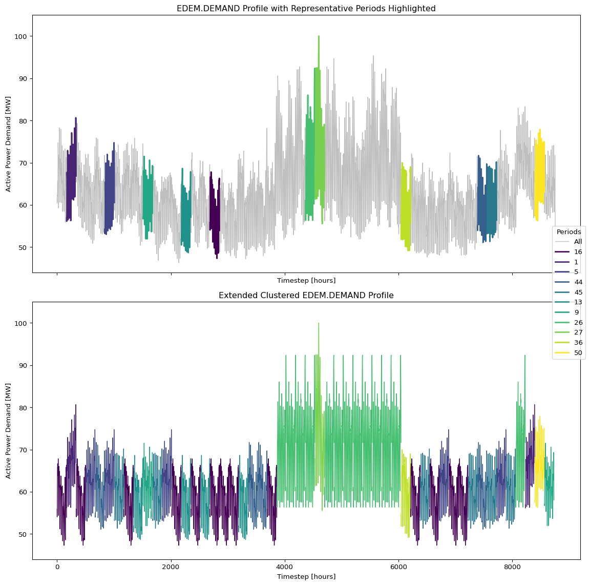
fig = dataset.plot_cem_profile(
    scenario='CEM_ESCE',
    profile='PV.SOLAR',
    y_label='Active Power Demand [MW]',
    out_file=None  # An image file will not be saved in this example
)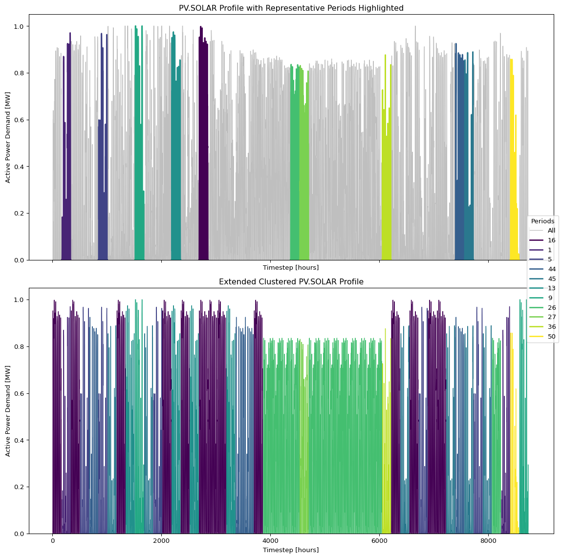
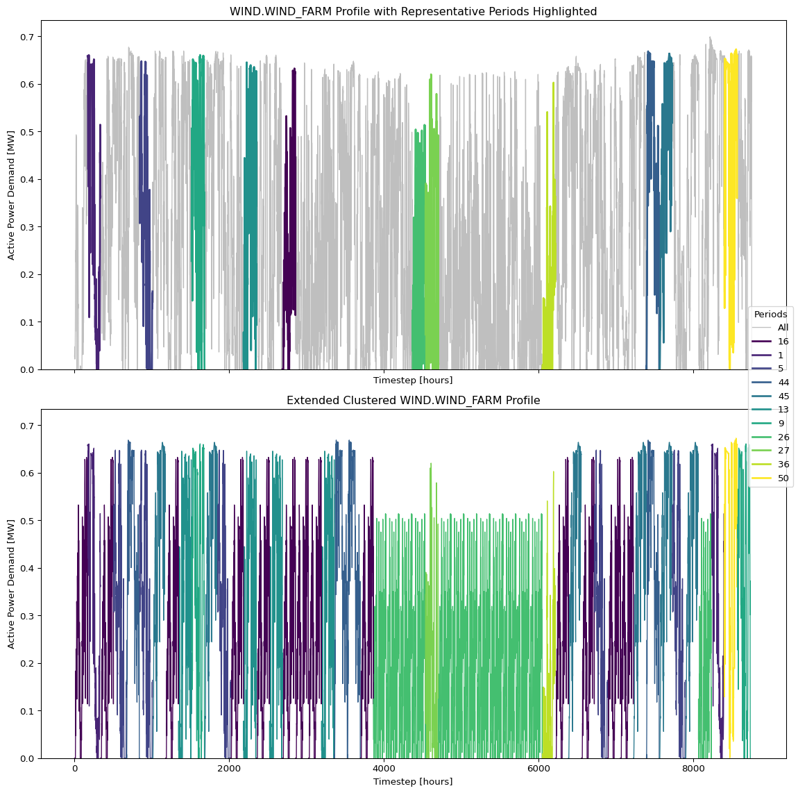
fig = dataset.plot_cem_profile(
    scenario='CEM_ESCE',
    profile='WIND.WIND_FARM',
    y_label='Active Power Demand [MW]',
    out_file=None  # An image file will not be saved in this example
)
6.2. Time-Domain Reduction Metadata
Users can access the number of iterations used in the k-means clustering process and the inertia of the clustered profiles, i.e. the "Sum of squared distances of samples to their closest cluster center, weighted by the sample weights if provided". See the scikit-learn docs for more details.
scen = dataset.get_scenario('CEM_ESCE')
scen.get_clustering_metadata()
{'NumberOfIterations': 5, 'Inertia': 8701.165052840484}